Simulink Model of a Lithium-Ion Battery

Michael Knauff, Jeffrey McLaughlin, Dr. Chris Dafis,

Dr. Dagmar Niebur, Dr. Pritpal Singh , Dr. Harry Kwatny, and Dr. Chika Nwankpa Simulink Model of a Lithium-Ion Battery for the

Hybrid Power System Testbed

ABSTRACT

This paper investigates the identification of model parameters for a Simulink model of the 60Ah Lithium Technology Corporation Lithium-ion battery used in the hybrid power systems testbed. Two experimental tests of the battery are presented, along with a method for deriving battery model parameters using these tests. A comparison between test data and simulation results shows a high degree of accuracy in the model.

1.INTRODUCTION

The Hybrid Power System Testbed is a small scale hardware demonstration currently being assembled at NAVSEA Philadelphia, that will combines several emerging technologies, and provides a means to experiment with advanced power management schemes, such as that described in (Kwatny et al. 2005).

The testbed consists of a variety of power sources and loads interconnected via a DC bus. The power sources include a Lithium-ion (Li-ion) battery and a diesel generator, with additional sources being considered for future implementation (ex. fuel cell). The loads consist of a rim-driven propulsion motor, a power processing unit capable of emulating a wide variety of loads, and two permanent magnet machines in a motor/generator configuration used to dissipate excessive power beyond the capabilities of the other two loads. The sources and loads are connected to the DC bus via several power electronic building block modules (Ericsen, Hingorani, and Khersonsky 2006).

In order to gauge the physical interaction of the developmental components during operation, a model of the testbed was created in Matlab/Simulink. The overall Simulink model of the testbed is described in greater detail in (Knauff et al. 2007). This paper provides a detailed look at the model of the testbed’s Li-ion battery. It also discusses in detail the derivation of the model parameters via testing of the physical device.

2.BATTERY MODEL

A variety of models exist that predict battery behavior to varying degrees of accuracy. A good overview of the different model types available is presented by Singh and Nallanchakravarthula (2005) The available models differ in both complexity and in the nature of the tests necessary to implement the models. The model selected for the testbed was proposed by Chen and Rincon-Mora (2006). It was chosen for its relative simplicity, including the advantage that a straightforward test is given to derive the associated model parameters.

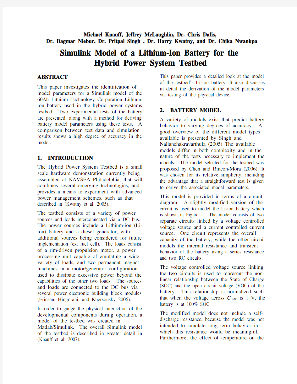
This model is provided in terms of a circuit diagram. A slightly modified version of the circuit is used to model the Li-ion battery which is shown in Figure 1. The model consists of two separate circuits linked by a voltage controlled voltage source and a current controlled current source. One circuit represents the overall capacity of the battery, while the other circuit models the internal resistance and transient behavior of the battery using a series resistance and two RC circuits.

The voltage controlled voltage source linking the two circuits is used to represent the non-linear relationship between the State of Charge (SOC) and the open circuit voltage (VOC) of the battery. This relationship is normalized such that when the voltage across C CAP is 1 V, the battery is at 100% SOC.

The modified model does not include a self-discharge resistance, because the model was not intended to simulate long term behavior in which this resistance would be meaningful. Furthermore, the effect of temperature on the

battery performance has not been accounted for in this version of the model due to the fact that the battery is expected to operate in a relatively narrow range of temperature conditions.

The circuit diagram in Figure 1 was implemented in Simulink by first finding an equivalent ordinary differential equation (ODE) describing the above circuit. The equation

1

1

1

1

1

1230

00

0()0

00()()CAP

TS

TS

TS TL

TL

TL

S C

R C C R C C

g x x x R ??????=?+???=+++??

???????????????

???

x

x u

y u

(1) describes the circuit diagram of Figure 1, where

R TS and C TS are the resistance and capacitance in the shorter time constant RC circuit, R TL and C TL are the resistance and capacitance in the longer time constant RC circuit, C CAP represents the overall capacitance of the battery, R S is the series resistance, and g (x ) is the non-linear function which maps SOC to VOC. The state vector x represents the voltages across C CAP , C TS , and C TL . The input u is the current entering the battery, and the output y is the voltage across the battery terminals. As noted above SOC is represented by the voltage v SOC across C CAP which ranges from 0 to 1 V, representing 0% to 100% battery capacity respectively.

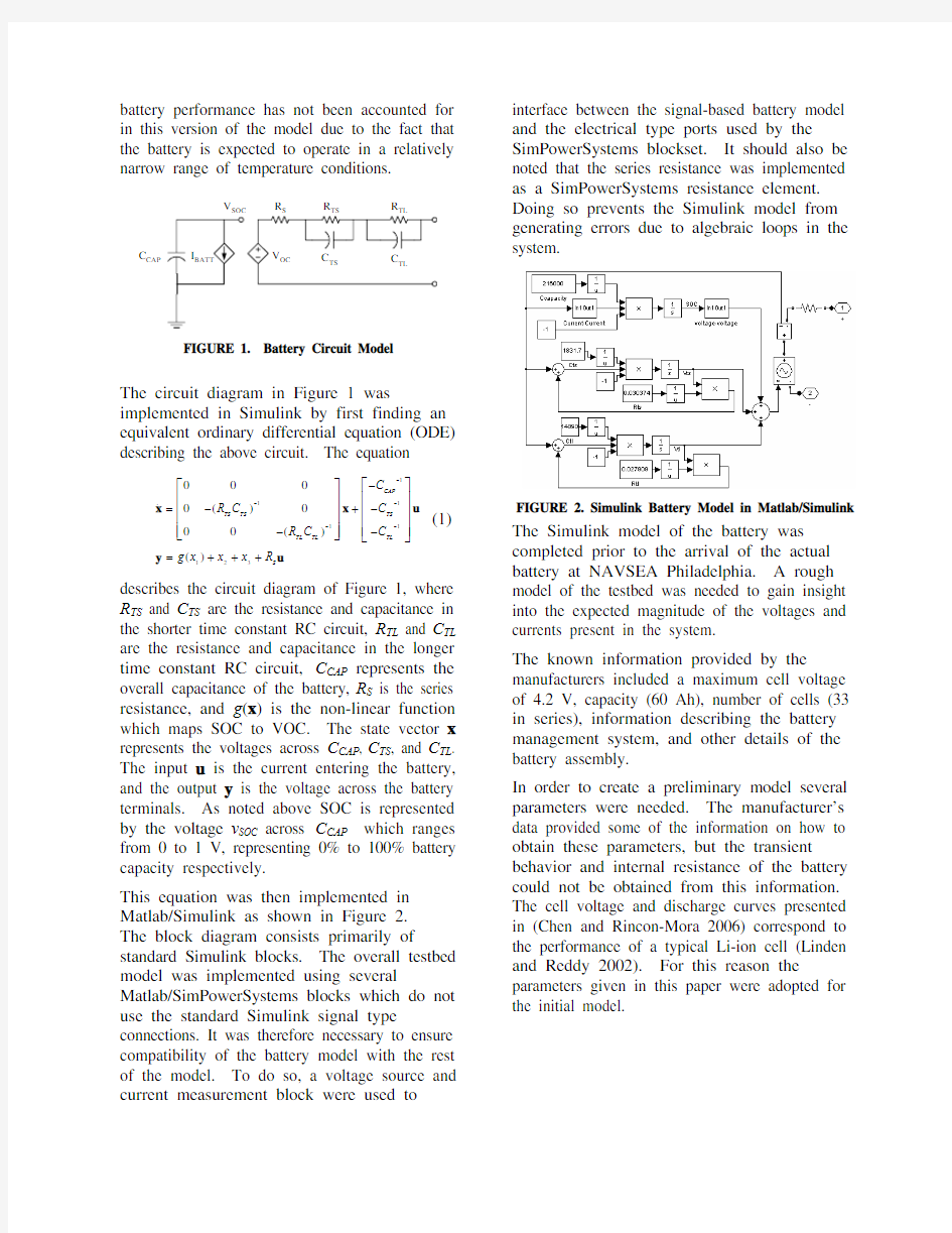
This equation was then implemented in Matlab/Simulink as shown in Figure 2. The block diagram consists primarily of standard Simulink blocks. The overall testbed model was implemented using several Matlab/SimPowerSystems blocks which do not use the standard Simulink signal type connections. It was therefore necessary to ensure compatibility of the battery model with the rest of the model. To do so, a voltage source and current measurement block were used to

interface between the signal-based battery model and the electrical type ports used by the SimPowerSystems blockset. It should also be noted that the series resistance was implemented as a SimPowerSystems resistance element. Doing so prevents the Simulink model from generating errors due to algebraic loops in the system.

The Simulink model of the battery was completed prior to the arrival of the actual battery at NAVSEA Philadelphia. A rough model of the testbed was needed to gain insight into the expected magnitude of the voltages and currents present in the system.

The known information provided by the manufacturers included a maximum cell voltage of 4.2 V, capacity (60 Ah), number of cells (33 in series), information describing the battery management system, and other details of the battery assembly.

In order to create a preliminary model several parameters were needed. The manufacturer’s data provided some of the information on how to obtain these parameters, but the transient behavior and internal resistance of the battery could not be obtained from this information. The cell voltage and discharge curves presented in (Chen and Rincon-Mora 2006) correspond to the performance of a typical Li-ion cell (Linden and Reddy 2002). For this reason the parameters given in this paper were adopted for

the initial model.

FIGURE 2. Simulink Battery Model in Matlab/Simulink

R R C CAP R V FIGURE 1. Battery Circuit Model

3.DERIVATION OF VOC–SOC

RELATIONSHIP

Once the actual battery arrived at NAVSEA Philadelphia, explicit model parameters had to be derived and employed in the model from battery tests. The first characteristic of the model to be experimentally derived was the non-linear function relating SOC to VOC.

To find an approximation for this function, a constant resistance discharge of the battery over

a safe discharge cycle was conducted. The battery is equipped with a battery management system (BMS) which, among other functionalities, automatically disconnects the battery terminals when the battery’s cell voltages are below a critical voltage level. This ensures that no permanent damage is inflicted on the battery. The discharge was executed until the point at which this mechanism triggers.

The setup used for this test is shown in Figure 3. Voltage and current at the battery terminals were monitored internally by the battery management system (BMS). This data is sampled once per second, and is made available via an RS232 port on the front of the battery assembly. Data was acquired using a serial connection and was stored as a text file for later analysis.

Upon completion of the test, the state of charge over the entire test period was found using the current data obtained from the test. Equation (2) was obtained from (1) and used to perform this calculation.

1

()(0)()

SOC SOC

CAP

v t v i d

C

τ

ττ

=?∫ (2)

Note that v SOC (0) should theoretically begin at 1 V for a fully charged battery. However, the measured voltage in each battery cell was roughly 4.09 V, while the manufacturer’s specifications listed a maximum cell voltage of 4.2 V. For this reason v SOC(0) was calibrated to be 0.9 V rather than 1 V.

The discharge-current data was numerically integrated (trapezoid rule) according to equation (2) yielding the SOC for each data point in the test. This data was then implemented in the model using an 11 point lookup table providing the corresponding values of VOC at the SOC values 0.0, 0.1, 0.2,…,1.0. A VOC value of 0 V was used for the 0.0 SOC value since the battery was not discharged to this point. Similarly a value of 138.6 V was used for 1.0 SOC corresponding to the manufacturer’s data for a fully charged cell multiplied by 33 cells.

After implementing this lookup table in the model, a simulation was used to demonstrate the improvement in this model compared with the initial model described above. Figure 4 shows a comparison between the actual data recorded during the discharge test, simulation results using the initial model, and simulation results for the refined model.

FIGURE 4. Battery Discharge Model Comparison

Blue – Experimental Data, Green – Initial Model

Red – Refined Model

FIGURE 3. Battery Test Setup

4.ESTIMATION OF RC AND SERIES

RESISTANCE PARAMETERS

After the SOC-VOC relationship had been derived the remaining model parameters were identified. A practical test for deriving these parameters is discussed in (Chen and Rincon-Mora 2006). The test involves a series of constant current discharge periods interspersed by a series of rest periods in which no current is drawn from the battery. Transient behavior of the battery is observed during these rest periods. This allows the model parameters to be derived at several points throughout the discharge cycle.

A similar test was conducted with one slight modification. Rather than using a set time interval for each pulse, the battery was discharged during the nine separate discharge cycles until a specific voltage v SOC was reached. Specified values were 0.9, 0.8, 0.7, …, 0.1 SOC. In the test setup shown in Figure 3 the resistive load was replaced by a programmable load capable of discharging the battery by drawing constant current. The rating of the available programmable load significantly limited the magnitude of the discharge current that could be applied in this test. The battery was therefore discharged for a significantly longer period of time compared to the test using the resistive load.

The load was programmed to toggle the current between 3.6 and 0 A based on a user trigger command. Each time the terminal voltage reached one of the predefined levels, the load was toggled and allowed to rest for approximately 25 minutes.

The battery was discharged down to a level of about 0.1 SOC and allowed to rest for one last transient period. Again, the battery was not fully discharged to avoid any potential damage to the battery. Throughout this process the current and terminal voltage of the battery were obtained via the RS232 output of the battery’s BMS.

After obtaining the test data the nine rest periods were separated and individually analyzed to obtain the model parameters. A technique for deriving these parameters is described by Schweighofer, Raab, and Brasseur (2003). However this technique is not completely automated because it requires some guidance in

selecting the two transient periods corresponding to the two RC circuits.

An alternative approach was instead taken which

utilized the Matlab Curve Fitting Toolbox.

Looking at the end of one discharge period at

the instant when the discharge current is turned

off, R S can be found by making the assumption

that the state vector remains constant in the

vicinity around this time instant. Equation (1) is

used to derive the equation

123

123

(()

(()

)

)

S C

t g x x x R

t g x x x

i

?

+

=+++

=++

y

y

(3)

where y(t-) is the terminal voltage prior to

turning off the discharge current and y(t +) is the

terminal voltage at the beginning of the rest

period. Then R S is given by

()()

S

C

y t y t

R

i

?+

?

= (4)

After finding R S the rest period can be analyzed.

Given that u in equation (1) is zero during this

period, the equation

1

12

1

3

()((0))(0)

(0)

TS TS

TL TL

R C

R C

y t g x x e

x e

?

?

=+

+

(5)

describes the terminal voltage during this interval.

To find x2(0) and x3(0) we consider the constant discharge period prior to the rest period. Using

equation (1) yields

()

()

1

()

22

1

()

33

()()

()()

TS TS

TL TL

t

R C

TS C TS C

t

R C

TL C TL C

x t x R i e R i

x t x R i e R i

τ

τ

τ

τ

?+

?+

=?+?

=?+?

(6)

where –τ is the time point at the beginning of the discharge period. Given that τ is sufficiently

large, the exponential components in equation

(6) are negligibly small at time t=0. Then Equation (6) reduces to

23(0)(0)TS C TL C

x R i x R i =?=?. (7)

Equation (5) is of the generic form

()bt dt y t k a e c e =+?+? (8)

The generic parameters k , a, b, c , and d were determined based on measurements of y (t ) and applying the Trust-Region algorithm of Matlab’s Curve Fitting Toolbox. Constraints on the parameters enforced positive values for k and negative values for a, b, c , and d . The battery model parameters were then derived from equations (5), (7), and (8) as

11TS C TL C TS TS TL TL a

R i c R i C R b C R d

=?

=?

=?=?

, (9) This method was used for each discharge period in the test. The resulting parameters are shown in Figures 5-9.

Rts as a function of SOC

SOC

R t s

FIGURE 8. R TS as a function of SOC

4

SOC

C t l

Ctl as a function of SOC

FIGURE 7. C TL as a function of SOC

Rtl as a function of SOC

SOC

R t l

FIGURE 6. R TL as a function of SOC

SOC

R s

Rs as a function of SOC

FIGURE 5. R S as a function of SOC

As noted in (Barsali and Ceraolo 2002), the RC circuit parameters are functions of the battery SOC. However, it should be noted that based on Figures 5-9 this variation is within an order of magnitude. Potentially, this parameter variation could be implemented in the Simulink model by replacing the parameter constant blocks with lookup tables.

Since it was desirable to keep the Simulink model as simple as possible, these parameters were instead implemented using the average of the parameters over the nine discharge cycles. A comparison of the resulting model with the test data is shown in Figures 10 and 11.

Figures 10 and 11 show a close match between the test data and simulation results (mean absolute percent error of 0.19 %), despite the fact that the averaged parameters were constant rather than functions of the SOC. Figure 11 presents a more detailed view of Figure 10, focusing on the time interval [3.75, 4]×104s and demonstrates that even when some steady state error is present the transient behavior of the model follows an almost identical path, only offset slightly from the actual system.

5. CONCLUSION

This paper investigates modeling and parameter identification of Li-ion batteries for use in numerical simulation in the Matlab/Simulink environment. A comparison of simulation and hardware testing results shows a high degree of accuracy with the selected battery model. In contrast to the technique proposed by Schweighofer, Raab, and Brasseur (2003) and utilized by Chen and Rincon-Mora (2006), where portions of the transient curve have to be identified manually, the technique investigated in this paper is completely automated. 6. ACKNOWLEDGMENTS

This work was supported in part by the Office of Naval Research Contract Number N00014-06-C-0041, the NSF-Navy Civilian Service (NNCS) Fellowship-Scholarship Program (NSF Aaward number #0549139), and ONR Contract #N65540-05-C-0028.

The authors would like to thank Lynn Petersen of ONR and John Metzer of NAVSEA-Philadelphia for their support and guidance during this effort.

x 10

4

Time (s)

V o l t a g e (V )

FIGURE 11. Comparison between simulation and test

data – detailed view

x 10

4

Time (s)

V o l t a g e (V )

FIGURE 10. Comparison between

simulation and test data

SOC

C t s

Cts as a function of SOC

FIGURE 9. C TS as a function of SOC

7.REFERENCES

Barsali, S., and M. Ceraolo. 2002. Dynamical models of lead-acid batteries: implementation issues. IEEE Transaction on Energy Conversion 17 (1):16-23.

Chen, Min, and G. A. Rincon-Mora. 2006. Accurate electrical battery model capable of predicting runtime and I-V performance. IEEE Transactions on Energy Conversion 21 (2):504-511.

Ericsen, T., N. Hingorani, and Y. Khersonsky. 2006. Power electronics and future marine electrical systems. IEEE Transactions on Industry Applications 42 (1):155-163.

Knauff, M. C., C. J. Dafis, D. Niebur, H. G. Kwatny, and C. O. Nwankpa. 2007. Simulink Model for Hybrid Power System Test-bed. Paper Accepted for Publication in Proceedings of IEEE Electric Ship Technologies Symposium, Arlington, VA, May 2007.

Kwatny, H. G., E. Mensah, D. Niebur, and C. Teolis. 2005. Optimal shipboard power system management via mixed integer dynamic programming. Proceedings of the IEEE Electric Ship Technologies Symposium, Philadelphia, PA, July 2005.

Linden, David, and Thomas B. Reddy. 2002. Handbook of batteries. 3rd ed. New York: McGraw-Hill.

Schweighofer, B., K. M. Raab, and G. Brasseur. 2003. Modeling of high power automotive batteries by the use of an automated test system. IEEE Transactions on Instrumentation and Measurement 52 (4):1087-1091.

Singh, P., and A. Nallanchakravarthula. 2005. Fuzzy logic modeling of unmanned surface vehicle (USV) hybrid power system. Proceedings of the 2005 Intelligent Systems Application to Power Systems, Arlington, VA, November 2005.

8.BIOGRAPHIES

Michael Knauff received the B.S.E. from the University of Hartford, Hartford, CT in 2003. He is currently pursuing his Ph.D. degree in electrical engineering at Drexel University, Philadelphia, PA. He is a student member of IEEE.Jeffrey McLaughlin received his B.E.E. at Villanova University in 2005, where he is currently in his last year of MSEE studies with a focus in power systems. While completing his graduate studies he has also held a research assistantship position funded by the Office of Naval Research. His research involves the construction and testing of an H-I-L hybrid power system testbed for unmanned surface vehicles. He is a member of Eta Kappa Nu, Tau Beta Pi, and a student member of IEEE.

Dr. Chris Dafis is an employee of NAVSEA-Philadelphia working in the Advanced Machinery Systems Integration branch (986). He received his B.S., M.S. and Ph.D. in Electrical Engineering and M.S. in Mathematics from Drexel University, in 1996, 1998, 2005, and 2002 respectively. His research interests are

in the areas of power systems protection, control, observability and stability as they apply to future Navy combatants. He is a member of IEEE, Eta Kappa Nu, and ASNE.

Dagmar Niebur received her Diploma in Mathematics and Physics from the University of Dortmund, Germany in 1984. She received her Diploma in Computer Science (1987) and her Ph.D. in Electrical Engineering (1994) from the Swiss Federal Institute of Technology, Lausanne, (EPFL) Switzerland. In 1997 she joined Drexel University's Electrical and Computer Engineering Department where she is currently an associate professor. Prior engagements included research positions at the Jet Propulsion Laboratory and EPFL. Her research focuses on intelligent information processing techniques for power system monitoring and control. In 2000, she received the NSF Career Award.

Pritpal Singh is Professor and Chairperson of the ECE Department, Villanova University. Dr. Singh received his B.Sc. from the University of Birmingham, U.K., and his Ph.D. from the University of Delaware. His research is focused on the SOC/SOH of batteries and fuel cells, photovoltaic devices and systems, and alternative energy sources.

Harry G. Kwatny received the B.S.M.E. degree, the M.S. degree in Aeronautics and

Astronautics, and the Ph.D. degree in Electrical Engineering from Drexel Institute of Technology, Philadelphia, PA, the Massachusetts Institute of Technology, Cambridge, and the University of Pennsylvania, Philadelphia, in 1961, 1962, and 1967, respectively. He joined the Department of Mechanical Engineering and Mechanics, Drexel University, Philadelphia, PA in 1966, where he

is currently the S. Herbert Raynes Professor of Mechanical Engineering. His research interests include modeling, analysis and control of nonlinear, parameter-dependent systems with specific applications to electric power systems and power plants, aircraft, spacecraft and ground vehicles. He has coauthored over 100 papers and

a monograph on non-linear control. He is also a coauthor of the software package TSi ProPac and a Mathematica package for nonlinear control system design and multibody mechanical system modeling.

Chika O. Nwankpa received the Magistr Diploma in Electric Power Ssystems from Leningrad Polytechnical Institute, USSR, in 1986, and the Ph.D. degree in the Electrical and Computer Engineering from the Illinois Institute of Technology, Chicago, in 1990. He is currently a Professor of Electrical and Computer Engineering and director of the Center for Electric Power Engineering (CEPE) at Drexel University, Philadelphia, PA. His research interests are in the areas of power systems and power electronics. Dr. Nwankpa is a recipient of the 1994 Presidential Faculty Fellow Award and the 1991 NSF Engineering Research Initiation Award.