Indoor Location Tracking in Non-line-of-Sight Environments Using a IEEE 802.15.4a Wireless Network

Postprint,In:Proceedings of the2009IEEE/RSJ International Conference on Intelligent Robots and Systems(IROS2009), pages552-557,St.Louis,USA,October2009

Indoor Location Tracking in Non-line-of-Sight Environments Using a IEEE802.15.4a Wireless Network

Christof R?hrig and Marcel Müller

Abstract—Indoor location tracking of mobile robots or transport vehicles using wireless technology is attractive for many applications.IEEE802.15.4a wireless networks o?er an inexpensive facility for localizing mobile devices by time-based range measurements.The main problems of time-based range measurements in indoor environments are errors by multipath and non-line-of-sight(NLOS)signal propagation. This paper describes indoor tracking using range measurements and an Extended Kalman Filter with NLOS mitigation.The commercially available nanoLOC wireless network is utilized for range measurements.The paper presents experimental results of tracking a forklift truck in an industrial environment.

I.I ntroduction

Indoor location tracking of mobile systems using wireless technology is attractive for many robotics and logistics applications.Wireless networks o?er an inexpensive facility for communication and localization of mobile devices.The new wireless network standard IEEE802.15.4a speci?es two optional signalling formats based on Ultra Wide Band (UWB)and Chirp Spread Spectrum(CSS)with a precision time-based ranging capability[1].Typical applications of IEEE802.15.4a are low power Wireless Personal Networks (WPAN)and Wireless Sensor Networks(WSN).A WSN consist of spatially distributed autonomous sensor nodes for data acquisition.Besides military applications and monitor-ing of physical or environmental conditions,robotics[2]and logistics[3]are typical application?elds of WSN.

The main problems of time-based range measurements in indoor environments are errors by multipath and non-line-of-sight(NLOS)measurements.For time-based range measurements,the direct line-of-sight(LOS)path which connects the transmitter and receiver is needed to calculate the range between them.In indoor environments,the LOS path can be blocked and the communications is conducted through re?ections and di?ractions.This phenomenon leads to positive bias in the range measurements and?nally causes errors in location tracking.A similar problem is multipath fading,which occurs in indoor environments,where the sig-nal propagates over multipath re?ections.The received signal is a superposition of the transmitted signal with di?erent delays.Multipath fading leads also to range measurements with positive bias.

This paper studies the tracking of a forklift truck using a nanoLOC WSN in conjunction with an Extended Kalman Filter and NLOS detection and mitigation.The nanoLOC C.R?hrig and M.Müller are with the Dortmund University of Applied Sciences and Arts,Department of Computer Science,Emil-Figge-Str.42, 44227Dortmund,Germany.Email:roehrig@https://www.360docs.net/doc/741590012.html, WSN,developed and distributes by Nanotron Technologies, o?ers ranging capabilities using CSS.The video attachment of the paper shows the movement of the forklift truck in a tracking experiment.

The paper extends the work we have presented in[4].The detection of NLOS conditions is studied and techniques for error mitigation are developed and compared by real-world experiments.The experimental results show the e?ectiveness of the proposed techniques.

II.R elated W ork

Up to now several kinds of localization techniques are developed for the use in wireless networks.A review of existing techniques is given in[5].These techniques can be classi?ed by the information they use.These informations are:connectivity,Received Signal Strength(RSS),Angle of Arrival(AoA),Time of Arrival(ToA),Round-trip Time of Flight(RToF)and Time Di?erence of Arrival(TDoA). Connectivity information is available in all kinds of wire-less networks.The accuracy of localization depends on the range of the used technology and the density of the beacons. In cellular networks Cell-ID is a simple localization method based on cell sector information.In infrastructure mode of a Wireless LAN(WLAN),the access point(AP)to which the mobile device is currently connected,can be determined since mobile devices know the MAC hardware address of the AP,which they are connected to.In a WSN with short radio range,connectivity information can be used to estimate the position of a sensor node without range measurement[6]. RSS information can be used in most wireless technolo-gies,since mobile devices are able to monitor the RSS as part of their standard operation.The distance between sender and receiver can be obtained with the Log Distance Path Loss Model described in[7].Unfortunately,the propagation model is sensitive to disturbances such as re?ection,di?raction and multi-path e?ects.The signal propagation depends on building dimensions,obstructions,partitioning materials and surrounding moving objects.Own measurements show,that these disturbances make the use of a propagation model for accurate localization in an indoor environment almost impossible[8].

AoA determines the position with the angle of arrival from?xed anchor nodes using triangulation.Drawback of AoA based methods is the need for a special and expensive antenna con?guration e.g.antenna arrays or rotating beam antennas.

ToA,RToF and TDoA estimate the range to a sender by measuring the signal propagation delay.The Cricket localiza-

tion system[9]developed at MIT utilizes a radio signal and an ultrasound signal for position estimation based on trilat-eration.TDoA of these two signals are measured in order to estimate the distance between two nodes.This technique can be used to track the position of a mobile robot[10].UWB o?ers a high potential for range measurement using ToA, because the large bandwidth(>500MHz)provides a high ranging accuracy[11].In[12]UWB range measurements are proposed for tracking a vehicle in a warehouse.IEEE 802.15.4a speci?es two optional signalling formats based on UWB and CSS with a precision ranging capability.Nanotron Technologies distributes a WSN with ranging capabilities using CSS as signalling format.

The main problems of time-based range measurements in indoor environments are errors by multipath and NLOS signal propagation.A method to mitigate these errors is the Biased Kalman Filter(BKF).In[13]a BKF is applied to mitigate range errors of time based measurement for localization of emergency callers in cellular networks.The e?ectiveness of the BKF is proven by simulations.

III.T he nano LOC L ocalization S ystem Nanotron Technologies has developed a WSN which can work as a Real-Time Location Systems(RTLS).The distance between two wireless nodes is determined by Symmetrical Double-Sided Two Way Ranging(SDS-TWR).SDS-TWR allows a distance measurement by means of the signal prop-agation delay as described in[14].It estimates the distance between two nodes by measuring the RToF symmetrically from both sides.

The wireless communication as well as the ranging methodology SDS-TWR are integrated in a single chip,the nanoLOC TRX Transceiver[15].The transceiver operates in the ISM band of2.4GHz and supports location-aware applications including Location Based Services(LBS)and asset tracking applications.The wireless communication is based on Nanotron’s patented modulation technique Chirp Spread Spectrum(CSS)according to the wireless standard IEEE802.15.4a.Data rates are selectable from2Mbit/s to 125kbit/s.

SDS-TWR is a technique that uses two delays,which occur in signal transmission to determine the range between two nodes.This technique measures the round trip time and avoids the need to synchronize the clocks.Time measurement starts in Node A by sending a package.Node B starts its measurement when it receives this packet from Node A and stops,when it sends it back to the former transmitter. When Node A receives the acknowledgment from Node B,the accumulated time values in the received packet are used to calculate the distance between the two stations.The di?erence between the time measured by Node A minus the time measured by Node B is twice the time of the signal propagation.To avoid the drawback of clock drift the range measurement is preformed twice and symmetrically.The signal propagation time t d can be calculated as

t d=(T1?T2)+(T3?T4)

4

,(1)

where T1and T4are the delay times measured in node A in

the?rst and second round trip respectively and T2and T3are

the delay times measured in node B in the?rst and second

round trip respectively.This double-sided measurement zeros

out the errors of the?rst order due to clock drift[14].

Based on the nanoLOC TRX transceiver and the micro-

controller ATmega128L,the nanoLOC WSN can be used

for developing location-aware and distance ranging wireless

applications[16].A mobile tag localizes itself by measuring

the distances to a set of anchors as reference points.The

anchors are located to prede?ned positions within a Cartesian

coordinate system.The tag position can be calculated by

trilateration.

IV.L ocation T racking U sing the E xtended K alman F ilter

By monitoring a dynamic system,the interior process state

such as position and velocity of mobile objects is not direct

accessible.The distance measurements are subject to errors

and noise.The Kalman Filter is an e?cient recursive?lter,

which estimates the state of a dynamic system out of a series

of incomplete and noisy measurements by minimizing the

mean of the squared error.It is also shown to be an e?ective

tool in applications for sensor fusion and localization.

The equations of the Kalman Filter fall into two groups:

“predictor equations”and“corrector equations”.Based on

the system input parameters,the current state estimate and

error covariance estimate are projected forward to obtain

the predicted a priori estimates for the next time step.

This operation is called“time update”.Following an actual

measurement is incorporated into the a priori estimate to

obtain an improved a posteriori estimate.In other words

the measurements adjust the predicted estimate at that time,

so that this operation is denoted“measurement update”.

As initial values for the primary estimation?x0and P0are

passed.After each time and measurement update pair,the

process is repeated with the previous a posteriori estimates.

This recursive nature is one of the appealing features of the

Kalman Filter and the essential advantage over other stochas-

tic estimation methods.The?lter recursively conditions the

current estimate on all of the past measurements and can be

used in real-time applications.

The basic?lter is well-established,if the state transition

and the observation models are linear distributions.In the

case,if the process to be estimated and/or the measurement

relationship to the process is speci?ed by a non-linear

stochastic di?erence equation,the Extended Kalman Filter

(EKF)can be applied.This?ltering is based on linearizing a

non-linear system model around the previous estimate using

partial derivatives of the process and measurement function.

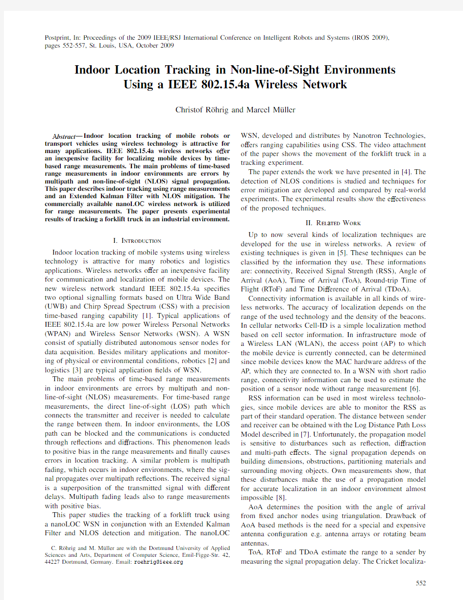
Fig.1shows a complete picture of the operations of

the EKF by presenting the speci?c predictor and corrector

equations.The time update projects the a priori state and

covariance estimates forward from time step to step.The

?rst task during the measurement update is to compute the

Kalman gain K k.The next step is to generate an a posteriori

state estimate?x k+1as the result of the?lter,in this case.

The ?nal step is to obtain the corresponding error covariance estimate P k +1for the next iteration.

Fig.1.Time update and measurement update equations of the Extended

Kalman Filter

A.Design of the Extended Kalman Filter

The Extended Kalman Filter is suitable to determine the x-and y-position of the mobile tag with the measured distances to at least three https://www.360docs.net/doc/741590012.html,ing the trilateration method the anchor distances r i are calculated as follow:

r i =√?

(p x ?a x ,i )2+(p y ?a y ,i )2,(2)where (a x ,i ,a y ,i )are the x-and y-positions of anchor i and

(p x ,p y )represents the x-and y-position of the mobile tag to be located.

To gain the unknown tag position,the equations in (2)are solved for p x and p y ,and are transformed in matrices:

H ·(?p x p y )?=z with H =????????????2·a x ,1?2·a x ,22·a y ,1?2·a y ,2......2·a x ,1?2·a x ,n 2·a y ,1?2·a y ,n

????????????,and z =????????????r 22?r 12+a x ,12?a x ,22+a y ,12?a y ,22...r n 2?r 12+a x ,12?a x ,n 2+a y ,12?a y ,n 2????????????,

(3)

where n is the overall number of anchor nodes.Eqn.3can be solved using the method of least squares:

(??p x

?p y )?=(H T H )?1H T ·z (4)For location tracking using EKF,Eqn.(3)needs only to

be solved for the initial estimate ?x 0.In this work the raw trilateration (3)is also used as reference.The EKF addresses the general problem of estimating the interior process state of a time-discrete controlled process,that is governed by non-linear di ?erence equations:

?x k +1=f (?x k ,u k ,w k ),

?y k +1

=h (?x k +1,v k +1).

(5)

The state vector contains the tag position x k =(p x ,p y )T .

The optional input control vector u k =(v x ,v y )T contains the desired velocity of the tag.These values are set to zero,if the input is unknown.The observation vector y k represents the observations at the given system and de?nes the entry parameters of the ?lter,in this case the results of the range measurements.The process function f relates the state at the

previous time step k to the state at the next step k +1.The

measurement function h acts as a connector between x k and y k .The notation ?x k and ?y k denotes the approximated a priori state and observation,?x k typi?es the a posteriori estimate of the previous step.Referring to the state estimation,the process is characterized with the stochastic random variables w k and v k representing the process and measurement noise.They are assumed to be independent,white and normal probably distributed with given covariance matrices Q k and R k .To estimate a process with non-linear relationships the equations in (5)must be linearized as follow:

x k +1≈?x k +1+A k +1·(x k ??x k )+W k +1·w k y k +1

≈?y k +1+C k +1·(x k +1??x k +1)+V k +1·v k +1,

(6)

where A k +1,W k +1,C k +1and V k +1are Jacobian matrices with

the partial derivatives:

A k +1=?f

?x (?x k ,u k ,0)W k +1=?f

?w (?x k ,u k ,0)C k +1=

?h

?x (?x

k +1,0)V k +1=

?h

?v (?x

k +1,0).(7)

Because in the analyzed system the predictor equation con-tains a linear relationship,the process function f can be

expressed as a linear equation:

x k +1=Ax k +Bu k +w k ,

(8)

where the transition matrix A and B are de?ned as:

A =(?1001)?,

B =

(?T 00T )?,

(9)

where T is the constant sampling time.

The observation vector y k contains the current measured distances:

y k =(?r 1···r n )?T .(10)The initial state estimate ?x 0is calculated based on (3).For

the subsequent estimation of the tag position (p x ,p y )the functional values of the non-linear measurement function h must be approached to the real position.The function h comprises the trilateration equations (2)and calculates the approximated measurement ?y k +1to correct the present estimation ?x k +1.The equation ?y k +1=h (?x k +1,v k +1)is given as:?????????????r 1...?r n ????????????=?????????????√?(?p x ?a x ,1)2+(?p y ?a y ,1)2...√?(?p x ?a x ,n )2+(?p y ?a y ,n )2

?????????????

+v k +1.(11)The related Jacobian matrix C k +1=?h

?x (?x

k ,0)describes the partial derivatives of h with respect to x :

C k +1=????????????????r 1??p x ??r 1??p y ......??r n ??p x

??r n ??p y

??????????????with ??r i ??p x =?p x ?a x ,i √(?p x ?a x ,i )2+(?p y ?a y ,i )2??r i ??p y =?p y ?a y ,i √(?p x ?a x ,i )2+(?p y ?a y ,i )2

.

(12)Given that h contains non-linear di ?erence equations the parameters r i as well as the Jacobian matrix C k +1must be calculated newly for each estimation.

B.Detection of NLOS range measurements

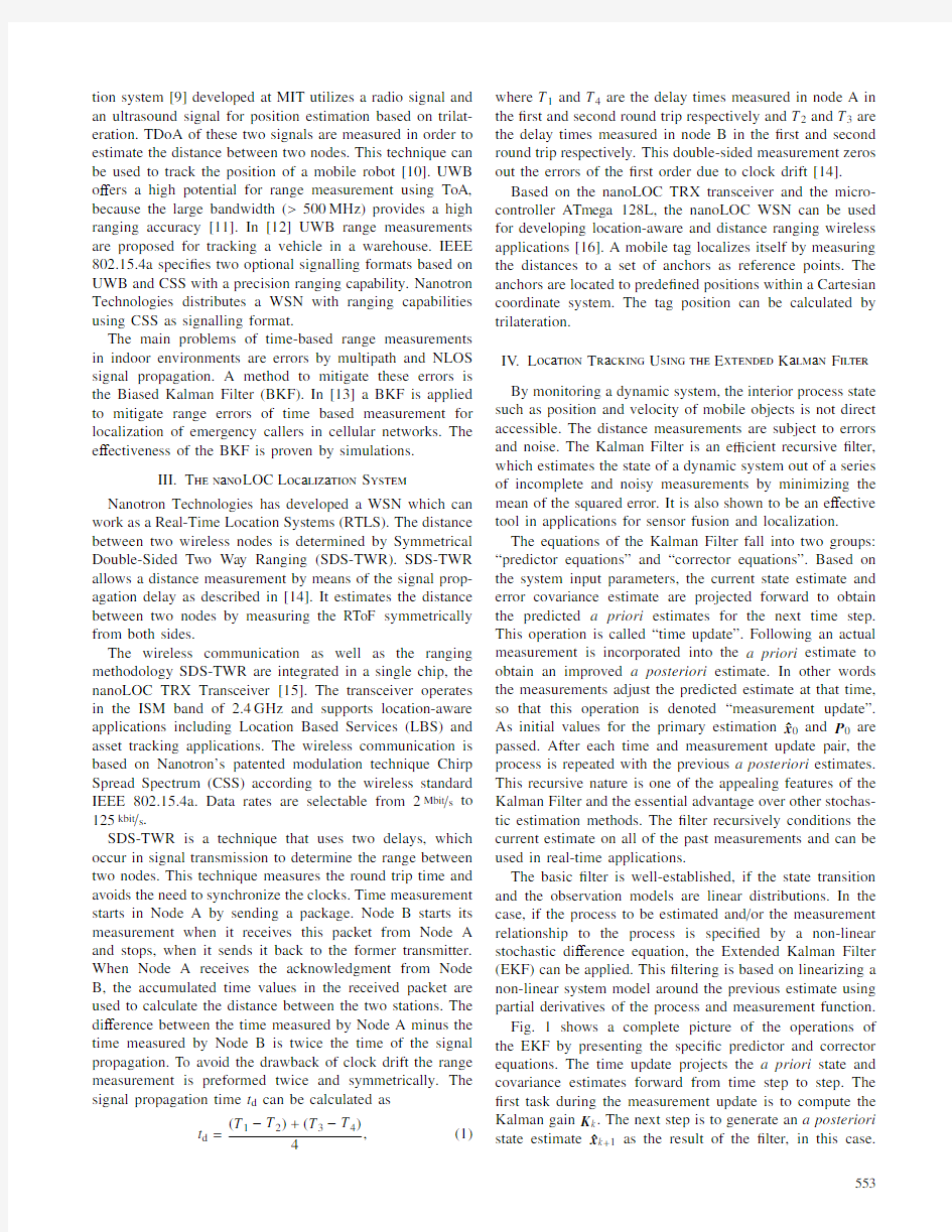
The range measurements can be modeled as

r i,k=d i,k+n i,k+e i,k,NLOS,(13) where r i,k is the range measurement to node i at sample time k,d i,k is the real distance,n i,k is the measurement noise and e i,k,NLOS is the measurement error due to NLOS. The measurement noise is modeled as Gaussian noise n i,k～N(0,σi),whereσi can be identi?ed by experiments.

Two di?erent techniques for NLOS detection are studied. Both methods use the time update of the Kalman Filter to estimate the position of the vehicle

?x k+1=Ax k+Bu k,(14) and to calculate the range estimates as

?r i,k+1=√?

(?p x,k+1?a x,i)2+(?p y,k+1?a y,i)2.(15)

The?rst method compares the range estimates to the real range measurements in order to detect NLOS:

?e i,k+1=r i,k+1??r i,k+1(16) Assuming small tracking errors?r i,k+1≈d i,k+1and comparing (13)with(16)leads to

?e i,k+1≈n i,k+e i,k,NLOS(17) NLOS is detected,if the error is positive and larger than a range error limit:

?e i,k+1≥e i,limit:NLOS

?e i,k+1

(18)

where the error limit e i,limit is obtained experimentally. The second technique use the standard deviation of the estimated range measurement errors(16)to detect NLOS as described in[13].Under NLOS condition,the signal propagation path changes quickly,when a vehicle moves. Owing to this fact,the standard deviation of the range measurement errors is signi?cantly larger in case of NLOS than in case of LOS condition.The standard deviation of the range errors(16)is estimated periodically in a?oating

window:

?σi=???

1

K

k

∑?

j=k?K+1

?e2

i,j

(19)

where K is the size of the?oating https://www.360docs.net/doc/741590012.html,paring?σi withσi detects NLOS conditions:

?σi≥γσi:NLOS

?σi<γσi:LOS

(20)

The parameterγcan be?nd out experimentally.γ>1 has to be chosen to reduce the probability of false alarm. The e?ectiveness of both techniques depends on the tracking performance of the EKF and on the quality of the initial state estimate?x0.C.Mitigation of NLOS range measurements

Two slightly di?erent methods for mitigation of NLOS range measurements have been studied.Both techniques use the Biased Kalman Filter.If NLOS is detected,the corre-sponding elements of the measurement covariance matrix R are increased:

R=

?

???

???

???

???

???

??

σ2

r,1

0 0

0σ2

r,2

···0

..

.

..

.

..

.

..

.

00···σ2r,n

?

???

???

???

???

???

??

(21)

The?rst technique(BEKF1)uses the estimated range error obtained from(16)to increase the covariance of R:

σ2

r,i

=

??

??

???

β?e iσ2

i

:NLOS

σ2

i

:LOS

,(22)

whereβis chosen by experiments to give a good tracking per-formance.The second method(BEKF2)uses the estimated covariance to increase the elements of R:

σ2

r,i

=

??

??

???

α?σ2

i

:NLOS

σ2

i

:LOS

,(23)

where?σ2

i

is obtained from(19)andαis chosen by experi-ments to give a good tracking performance.

These techniques are compared with an EKF,which dis-cards NLOS range measurements.The NLOS measurements are discarded by adapting the output equation of the EKF. Only LOS measurements are included in y k and C k of(10) and(12).

V.E xperiment R esults and P erformance A nalysis

A.Experimental Setup

In a test series,the position of a forklift truck is tracked using the described method.The experiments are carried out at a demonstration storage of the Fraunhofer-Institute for Ma-terial Flow and Logistics in Dortmund Germany.The forklift truck moves in automatic mode along a half oval course. It is controlled by laser triangulation,which has a tracking performance better than a few cm.The video attachment of the paper shows the forklift truck moving along this course. The standard nanoLOC development kit which contains?ve sensor boards with sleeve dipole omnidirectional antennas is utilized for the experiment.Four anchor nodes are placed at the edges of the course.The sampling time T is chosen to 0.3s.Several experiments with di?erent NLOS conditions have been performed to evaluate the e?ectiveness of the proposed techniques.The measured range data are logged into a?le for later analysis.The proposed NLOS mitigation techniques are implemented in Matlab and are evaluated o?ine.

B.Parameter Tuning

The e?ect of the Kalman estimation depends signi?cantly on the parameters of the covariance matrices.To preferably gain an exact estimation,appropriate values for the process noise covariance Q k and the measurement noise covariance

R k must be detected.The process noise covariance represents the accuracy of the estimates for the interior process state.The measurement noise covariance depends directly on the environment of the range measurements.Several experiments with di ?erent anchors in a static environment show covari-ances in a range between 0.0216m 2and 0.354m 2.The mea-surement noise covariance is chosen with σ2i =0.1328m 2

as mean variance of all experiments.These two matrices have a large impact in progress of the error covariance estimate P k ,whose initial value is assumed to P 0=I ·10?2.

The parameters have been chosen by experiments to e i ,limit =5m,α=1,K =10,β=1m ?1and γ=3.These parameters show the best tracking performance for the associated methods.C.Experimental Results

Several experiments with di ?erent NLOS conditions have been performed to evaluate the e ?ectiveness of the proposed techniques.In all experiments anchor node 1is blocked manually with a sheet of metal several times during the motion of the forklift truck.The results of three experiments are summarized in Table I.Fig.2to Fig.5show the results of the ?rst experiment.The LOS was blocked manually several times in intervals of 5s.The red line shows the course of the forklift truck,which is controlled by laser triangulation.The raw trilateration is shown with green dots and calculated with Eqn.(4).Owing to the measurement noise of the range measurements,the raw trilateration is spread over the whole area.In all ?gures the raw trilateration is calculated without NLOS mitigation.Owing to this fact,the measured distances to anchor 1are too large,and the estimated positions are displaced towards larger values of x and y .Several of the trilateration points are out of the range of the axis.

Fig.2shows the results of the EKF without NLOS mitigation.The estimated position of the EKF is shown as blue line.Fig.2shows that NLOS leads to worse tracking performance,if an unmodi?ed EKF is applied.NLOS dis-places the estimated position in the opposite direction of the related anchor node.

position x (m)

p o s i t i o n y (m )

Fig.2.Tracking results of EKF without NLOS mitigation

The same data are used for the EKF and NLOS measure-ment exclusion shown in Fig.3.The tracking performance is much better than using an unmodi?ed EKF.In environments with a large number of NLOS conditions,the lack of LOS measurements can lead to estimation failure.In this setup

position x (m)

p o s i t i o n y (m )

Fig.3.Tracking results of EKF with NLOS measurement rejection

measurements with ?e i >10m are discarded.Lowering this limit lead to a complete failure of the location estimation.In cases where the tracking error becomes high,the range error estimates increases and all measurements are discarded.The BEKF uses both LOS and NLOS range measure-ments.NLOS measurements are less weighted than LOS measurements.Fig.4.shows the results from using BEKF with NLOS mitigation method BEKF1.The tracking

perfor-position x (m)

p o s i t i o n y (m )

Fig.4.Tracking results of BEKF1

mance is better than using an unmodi?ed EKF.The ?lter reacts immediately after detecting a NLOS condition.

Fig.5shows the results from using NLOS mitigation method BEKF2.The tracking performance is slightly better than method BEKF1.Fig.6shows the distribution of the

position x (m)

p o s i t i o n y (m )

Fig.5.

Tracking results of BEKF2

true range errors e i of the four anchor nodes.The distribution shows NLOS condition in anchor node 1and biased range errors in the other anchor nodes,which may be caused by multipath signal propagation.

range error (m) range error (m)f r e q u e n c y

range error (m)f r e q u e n c y

range error (m)

f r e q u e n c y

Fig.6.Histogram of true range errors e i

TABLE I

M ean absolute error and standard deviation

#EKF EKF disc.BEKF1BEKF2mean abs error 11,760,590,470,28standard deviation 1,361,071,210,91mean abs error 20,510,510,460,38standard deviation 0,810,810,780,75mean abs error 3

0,560,580,510,58standard deviation

1,52

1,55

1,43

1,55

The mean absolute error and the standard deviation of the errors are listed in Table I,for three experiments.In the ?rst experiment LOS was blocked several times in intervals of 5s.In experiment 2LOS is blocked for 4s just before and after the curve.In the third experiment LOS is blocked for 8s in the second half of the course.BEKF2shows the best tracking performance in most cases.

VI.C onclusions

In this paper,location tracking of an forklift truck using range measurements and Biased Extended Kalman Filtering with NLOS mitigation is described.The main source for ranging errors in indoor environments is NLOS and multi-path signal propagation.Two di ?erent techniques for NLOS mitigation have been evaluated and compared with an un-modi?ed EKF and with an EKF with NLOS measurement exclusion.Discarding NLOS measurements is the easiest way to handle NLOS range measurements.In environments with a large number of NLOS conditions,the lack of LOS measurements may lead to estimation failure.In cases where the tracking error becomes high,the range error estimates increases and all measurements are discarded.

The BEKF uses LOS as well as NLOS range measure-ments.NLOS measurements are less weighted than LOS measurements.The ?rst technique (BEKF1)uses the esti-

mated range error directly.The second technique (BEKF2)calculates the standard deviation of the range errors.Both techniques are more robust than EKF and o ?er better track-ing performance.The ?rst technique reacts faster on NLOS.The second technique leads to a slightly better tracking performance.

R eferences

[1]Z.Sahinoglu and S.Gezici,“Ranging in the IEEE 802.15.4a Stan-dard,”in Proceedings of the IEEE Annual Wireless and Microwave Technology Conference,WAMICON ’06,Clearwater,Florida,USA,Dec.2006,pp.1–5.

[2]J.Graefenstein,A.Albert,and P.Biber,“Radiation Pattern Correlation

for Mobile Robot Localization in Low Power Wireless Networks,”in Proceedings of the 2009IEEE International Conference on Robotics and Automation ,May 2009,pp.3545–3550.

[3]S.Spieker and C.R?hrig,“Localization of Pallets in Warehouses using

Wireless Sensor Networks,”in Proceedings of the 16th Mediterranean Conference on Control and Automation ,Corsica,France,Jun.2008,pp.1833–1838.

[4] C.R?hrig and S.Spieker,“Tracking of Transport Vehicles for

Warehouse Management using a Wireless Sensor Network,”in 2008IEEE /RSJ International Conference on Intelligent Robots and Systems (IROS 2008),Nice,France,Sep.2008,pp.3260–3265.

[5]M.V ossiek,L.Wiebking,P.Gulden,J.Wieghardt,C.Ho ?mann,and

P.Heide,“Wireless Local Positioning,”Microwave Magazine ,vol.4,no.4,pp.77–86,Dec.2003.

[6]L.Hu and D.Evans,“Localization for Mobile Sensor Networks,”in

Proceedings of the 10th Annual International Conference on Mobile Computing and Networking ,2004,pp.45–57.

[7]N.Patwari,A.O.Hero,M.Perkins,N.S.Correal,and R.O’Dea,

“Relative Location Estimation in Wireless Sensor Networks,”IEEE Transactions on Signal Processing ,vol.51,no.8,pp.2137–2148,2003.

[8] C.R?hrig and F.Künemund,“Estimation of Position and Orientation

of Mobile Systems in a Wireless LAN,”in Proceedings of the 46th IEEE Conference on Decision and Control ,New Orleans,USA,Dec.2007,pp.4932–4937.

[9]N. B.Priyantha, A.K.L.Miu,H.Balakrishnan,and S.Teller,

“The Cricket Compass for Context-aware Mobile Applications,”in Proceedings of the 7th Annual International Conference on Mobile Computing and Networking ,Rome,Italy,Jul.2001,pp.1–14.

[10]P.Alriksson and A.Rantzer,“Experimental Evaluation of a Distributed

Kalman Filter Algorithm,”in Proceedings of the 46th IEEE Confer-ence on Decision and Control ,New Orleans,Dec.2007,pp.5499–5504.

[11]S.Gezici,Zhi Tian,G.Giannakis,H.Kobayashi,A.Molisch,H.Poor,

and Z.Sahinoglu,“Localization via Ultra-wideband Radios:A Look at Positioning Aspects for Future Sensor Networks,”Signal Processing Magazine ,vol.22,no.4,pp.70–84,Jul.2005.

[12]J.Fernández-Madrigal, E.Cruz,J.González, C.Galindo,and

J.Blanco,“Application of UWB and GPS Technologies for Vehicle Localization in Combined Indoor-Outdoor Environments,”in Proceed-ings of the International Symposium on Signal Processing and its Applications ,Sharja,United Arab Emirates,Feb.2007.

[13] B.L.Le,K.Ahmed,and H.Tsuji,“Mobile Location Estimator with

NLOS Mitigation Using Kalman Filtering,”in Proceedings of the Wireless Communications and Networking Conference ,vol.3,Mar.2003,pp.1969–1973.

[14]“Real Time Location Systems (RTLS),”Nanotron Technologies

GmbH,Berlin,Germany,White paper NA-06-0248-0391-1.02,Apr.2007.

[15]“nanoloc TRX Transceiver (NA5TR1),”Nanotron Technologies

GmbH,Berlin,Germany,Datasheet NA-06-0230-0388-2.00,Apr.2008.

[16]“nanoloc Development Kit User Guide,”Nanotron Technologies

GmbH,Berlin,Germany,Technical Report NA-06-0230-0402-1.03,Feb.2007.