A Deterministic Finite State Automaton for the Oriya Negative Verbal Forms

A Deterministic Finite State Automaton for the Oriya Negative Verbal Forms

Kalyanamalini Sahoo

ILTS Project

Dept. of Management Studies

Indian Institute of Science

Bangalore- 560012

kalyani@mgmt.iisc.ernet.in

Abstract

This paper discusses the processing of negative verbal forms in Oriya in a deterministic Finite State Automaton. A morphologically agglutinative language like Oriya has ‘phrasal’ or ‘constituent’ negation, where tense, aspect etc. impose restrictions on NEG marking. Negation can be marked by various NEG morphemes in various positions of the verbal form, but is marked only once. That is, the occurrence of a NEG morpheme restricts the occurrence of any other NEG marker in the verbal form. Such multiple positional slots for the NEG morpheme with respect to tense, aspect poses constraint for the processing of the string by FSA. The FSA being a unidirectional machine, cannot backtrack, and thus, cannot account for such mutual exclusiveness of the items if all the three NEG items are available in a single chart. So, to account for this problem, we propose different types of processing for the different positional slots of NEG morphemes.

1. Introduction

Morphological analysis of words is a basic tool for automatic language processing, and indispensable when dealing with agglutinative languages like Oriya. In this context, some applications, like spelling correction, do not need more than the segmentation of each word into its different component morphemes along with their morphological information. However, there are other applications such as lemmatization, tagging, phrase recognition, and determination of clause boundaries, which need an additional morphosyntactic parsing of the whole word. This work proposes a model for designing a morphological analyzer for Oriya negative verbal forms. This will not involve doing anything on the computer (for now!), just drawing out a finite-state machine that accepts valid sequences of morphemes in a negative verbal form and rejects invalid ones. 1.1 Negation

Negation is generally contrasted with affirmation, providing a polarity distinction between positive and negative. Languages differentiate between clausal and phrasal negations. In some languages, negation is primarily viewed as a clausal concept, in the sense that it would be unaffected by verbal categories like tense, aspect and evidentiality (or mood), i.e. English. A language like Oriya has phrasal or constituent negation, where tense, aspect etc. impose restrictions on NEG marking.

Languages use different devices to mark negation. Oriya has NEG affixes as well as NEG verbs. Negation can be marked by bound inflection on the verb, or can surface as an auxiliary verb. Finite and nonfinite verbal forms in Oriya have their own ways for being marked for negation. Negation can be marked by various NEG morphemes in various positions of the verbal form, but is marked only once. That is, the occurrence of a NEG morpheme restricts the occurrence of any other NEG marker in the verbal form. It can be marked at the beginning, middle or at the end of a finite verbal form, by the morphemes na-, naahan, and –ni/ naahin, respectively; while in non-finite verbal forms, the NEG affix na occurs invariably in a position immediately preceding the verbal root.

Such multiple positional slots for the NEG morpheme with respect to tense, aspect poses constraint for the processing of the string by a deterministic Finite State Automaton (FSA). The FSA being a unidirectional machine, cannot backtrack, and thus, cannot account for such mutual exclusiveness of the items if all the three NEG items are available in a single chart, and may over-generate. So, to account for this problem, we propose different types of processing for the different positional slots of NEG morphemes.

The remainder of this paper is organized as follows. Section 2 gives a brief description of the Oriya verbal forms. Section 3 and section 4 discuss NEG verb and NEG affixes, respectively. Section 5 summarizes the

NEG markers and the available positional slots for the NEG markers. Section 6 describes the architecture for morphological processing, specifies the phenomena covered by the analyzer, explains its design criteria, and presents the processing details. Finally, the paper ends with some concluding remarks.

2. Oriya verbal forms

Oriya is a syntactically head-final and morphologically agglutinative language. A number of morphemes carrying different grammatical functions get affixed to the verbal root to make a verbal form. The major inflectional subsystems that cluster around the verb are: tense, aspect, agreement markers, negation markers, auxiliary morpheme etc. Oriya verbal forms typically contain a sequence of morphemes followed by a verbal root, as in (1)-(2).

(1) (mun) khaa-u-th-il-i

I eat-PROG-AUX-PAST-1st sg

‘(I) was eating’

(2) (se) ne-i-th-ib-a

s/he take- PERF-AUX-PAST-3rd sg

‘(S/he) would have taken.’

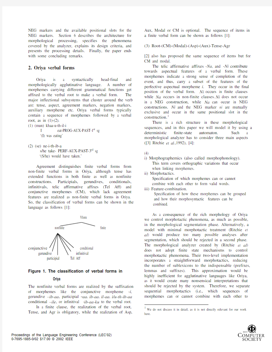
Agreement distinguishes finite verbal forms from non-finite verbal forms in Oriya, although tense has extended functions in both finite as well as nonfinite constructions. Participials, gerundives, conditionals, infinitivals, telic affirmative affixes (Tel Aff) and conjunctive morphemes (CM), which lack agreement features are realized as non-finite verbal forms in Oriya. So, the classification of verbal forms can be shown in the language as follows [1]:

Vform

nonfinite finite

conjunctive conditional

gerundive infinitival

participial Tel Aff

Figure 1. The classification of verbal forms in

Oriya

The nonfinite verbal forms are realized by the suffixation of morphemes like the conjunctive morpheme -i, gerundive –ib-aa, participial –aa, ib-aa, il-aa, i/u-th-ib-aa conditional –ile, or infinitival -ib-aa-ku to the verbal root.

In a finite clause, the realization of the verbal root, Tense, and Agr is obligatory, while the realization of Asp, Aux, Modal or CM is optional. The sequence of items in

a finite verbal form can be shown as follows [1]:

(3) Root-(CM)-(Modal)-(Asp)-(Aux)-Tense-Agr

[2] also has proposed the same sequence of items but for CM and modal.

The telic affirmative affixes-Na, and -Ni contribute towards aspectual features of a verbal form. These morphemes indicate a strong sense of completion of the event, and thus, carry a subset of the features of the perfective aspectual morpheme i. They occur in the final position of the verbal form. Ni occurs in finite clauses while Na occurs in non-finite clauses. Ni does not occur in a NEG construction, while Na can occur in NEG constructions. Ni and the NEG marker ni are mutually exclusive and occur in the same positional slot in the construction.1

There is a rich structure in these morphological sequences, and in this paper we will model it by using a deterministic finite-state automaton. Such a morphological analyzer has to consider three main aspects ([3] Ritchie et al.,1992), [4]:

(4)

i) Morphographemics (also called morphophonology).

This term covers orthographic variations that occur

when linking morphemes.

ii) Morphotactics.

Specification of which morphemes can or cannot

combine with each other to form valid words.

iii) Feature-combination.

Specification of how these morphemes can be grouped and how their morphosyntactic features can be

combined.

As a consequence of the rich morphology of Oriya we control morphotactic phenomena, as much as possible, in the morphological segmentation phase. Alternatively, a model with minimal morphotactic treatment (Ritchie et al) would produce too many possible analyses after segmentation, which should be rejected in a second phase. The morphological analyzer created by (Ritchie et al) does not adopt finite state mechanisms to control morphotactic phenomena. Their two-level implementation incorporates a straightforward morphotactics, reducing the number of sublexicons to the indispensable (prefixes, lemmas and suffixes). This approximation would be highly inefficient for agglutinative languages like Oriya, as it would create many nonsensical interpretations that should be rejected by the system. Therefore, we separate sequential morphotactics (i.e., which sequences of morphemes can or cannot combine with each other to 1We do not discuss it in detail, as it is not directly relevant for our work here.

form valid words), which will be recognized by means of

continuation classes, and non-sequential morphotactics like long-distance dependencies that will be controlled by the word-grammar.

3. The Negative verb

In Oriya, negation can surface as an auxiliary verb, that is, the negative marker has some of the usual properties of a verb, such as (tense)2, Agr. The Oriya negative auxiliaries, naahin and nuhai / nuhen seem to be derived from Sanskrit naasti and na bhavati, respectively. They correspond to the Oriya copular auxiliaries achh and aT. Like achh and aT, they occur in finite constructions only and have regular conjugations in the present tense. Each of them has a separate conjugation and is not used for the other.

naahin ‘not to be’, or ‘not to remain’ is the negative correlate of the copular auxiliary achhi‘to be’, or ‘to remain’, and thus behaves the similar way as achhi. Like achhi,it can be used as a copular auxiliary (like a main verb) as well as an auxiliary affix. Consider the following: (5) aaji se juga naahin ki

today that age be NEG -3rd sg PRT

se raajaa naahaanti

that king be NEG [+Hon]3rd sg

‘Today that time is not there, nor that king.’

(6) se kheL-u-naahin

he play-PROG- be NEG 3rd sg

‘He is not playing’.

In (5), naahin and naahaanti are used as independent verbs, while in (6) naahin functions as an auxiliary affix.

nuhen (short for nuhai from na+huai) is solely a full verb (as opposed to a bound morpheme). That is, it can be used only as an independent copula. It is the negative correlate of the equative copula verb aTe or aTai.

When the predicate is an adjective and denotes something habitual, usually nuhen is used. E.g.

(7) mun andha nuhen

I blind be NEG 1st sg

‘I am not blind.’

(8) mo baapaa Daaktara nuhanti

my father doctor be NEG [+Hon]3rd sg

‘My father is not a doctor.’

(9) kaban paark maaDraasre nuhen, baangaalor-re

Cubbon park Madras-PP be NEG 3rd sg, Bangalore-PP ‘Cubbon park is not in Madras, but in Bangalore.’

2 The negative auxiliaries appear in present tense only. (10) himaaLaya bhaaratara purbare nuhen,

Himalaya India’s east-PP be NEG 3rd sg

utarare (aTe)

north-PP (be 3rd sg)

‘The Himalayas is not on the east of India, it is on the north.’

Note that although the affirmative copula aTe can be dropped, nuhen cannot be dropped:

(11) a. se chhataaTaa mora (aTe)

that umbrella mine (be 3rd sg)

‘That umbrella is mine.’

b. se chhataaTaa mora nuhen

that umbrella mine be NEG 3rd sg

‘That umbrella is not mine.’

So, we can say that although dropping of the affirmative copula is very common in Oriya, dropping of the negative copula is not allowed.

4. NEG affixes

In Oriya, negation can be marked by bound inflection on the verb. The NEG morpheme has various morphological realizations in various positions of the verbal form. In finite constructions, negation can be marked at the beginning, middle or at the end of the verbal form, by the morphemes na-, naahan and –ni/ naahin3, respectively.4na is used in finite as well as in nonfinite constructions, while the other two NEG markers are used in finite constructions only.

4.1 NEG marking in nonfinite verbal forms

In a nonfinite construction, the NEG morpheme occurs being prefixed to the verbal root. Consider the following examples.

(12) se nakhaai chaaligalaa

he NEG-eat-CM walk-CM-go-PAST-3rd sg

‘He went away without eating.’

(13) mun nakaripaarile aau

I NEG-do-CM-modal-COND more

kaNa karibi

what do-FUT 1st sg

‘What shall I do if I cannot!’

3ni is the contracted form of naahin.

4 In the case of verbal adjectives, the NEG marker a occurs being prefixed to the verbal root. E.g.

(1) a-jaNaa loka (2) a-sijhaa anDaa

NEG-known man NEG-boiled egg

‘Unknown person.’ ‘Unboiled egg.’

In (12)-(13), the NEG marker always occurs in a position immediately preceding the verbal root. It cannot occur in any other position of the verbal form.

4.2 NEG marking in finite verbal forms

Consider NEG marking in finite constructions. The NEG marker can occur in various positions of the verbal form.

NEG in the initial position:

NEG morpheme can occur being prefixed to the verbal root, e.g.

(14) se na-khaa-i-paar-e

s/he NEG-eat- CM-modal-AGR

‘S/he may not eat.’

NEG can occur immediately preceding the Aux:

(15) mun jaainathaanti

I go- ASP perf-NEG-AUX-TENSE hyp-AGR

‘I would not have gone.’

(16) se jaa-i-na-th-il-aa

he root-ASP perf-NEG-AUX-TENSE past-AGR

‘He had not gone.’

In the presence of a main verb, modal and an Aux, the NEG marker usually occurs in a position immediately preceding the Aux; e.g.

(17) *se nakhaa-i-paar-i-th-ant-aa

he NEG-eat- CM-can-ASP-AUX-TENSE-AGR

‘He could not have eaten.’

(18) se khaa-i-paar-i-na-th-ant-aa

he eat-CM-can-ASP-NEG-AUX-TENSE-AGR

‘He could not have eaten.’

NEG at the place of Aux:

As we discussed earlier, the NEG auxiliary occurs in the same positional slot as that of the Aux morpheme. Being the NEG -correlate of the copular auxiliary morpheme achh, it can be used in PRES tense only. As we discussed above in (6), this NEG marker naahin is the co-relate of the aux-affix (not aux copula), and thus, is realized as an affix. E.g.

(19) mun khaaunaahin

I eat-ASP-NEG-AGR

‘I am not eating.’

(20) tume khaaunaahan

you eat-ASP-NEG-AGR

‘You are not eating.’

(21) mun khaaipaarunaahin

I eat-CM-modal-ASP-NEG-AGR

‘I am not able to eat.’ (22) tume khaaipaarunaahan

you eat-CM-modal-ASP-NEG-AGR

‘You are not able to eat.’

NEG at the final position of the verbal form:

The NEG morpheme at the final position is realized as ni/naahin. E.g.

(23) semaane khaanti-ni/naahin

they eat-Tense-AGR-NEG

‘They do not eat.’

(24) se khaailaa-ni/naahin

he eat-Tense- AGR-NEG

‘He did not eat.’

(25) se khaaiba-ni/naahin

he eat-Tense- AGR-NEG

‘He will not eat.’

(26) mun khaaipaaribi-ni/naahin

I eat- CM-Mod-Tense- AGR-NEG

‘I cannot eat.’

Note that although it resembles the NEG Aux naahin, it is different from that. Compare (19)-(21) with (23)-(26). The NEG Aux realizes the Agr features in (19)-(21), which is not found in the case of the NEG affix as in (23)-(26).

However, in the presence of ni,the construction cannot have aspectual realization as ni does not co-occur with Asp (or Asp-Aux) morphemes. In the presence of an Asp (or Asp-Aux) morpheme in the verbal form, the other neg marker na is realized, not ni. E.g.

(27) a. se khaa-u-na-th-il-aa

s/he eat-Asp-NEG-AUX-TENSE-AGR

‘S/he was not eating.’

b. *se khaa-u-th-il-aa-ni

s/he eat-Asp-AUX-TENSE-AGR-NEG

‘S/he was not eating.’

(28) a. se khaa-i-na-th-ib-a

s/he eat-ASP-NEG -AUX-TENSE-AGR

S/he will not have eaten.’

b.*se khaa-i-th-ib-a-ni

s/he eat-ASP-AUX-Tense-AGR-NEG

‘S/he will not have eaten.’

It indicates that ni might be the negative correlate of the telic affirmative affix Ni, which also does not co-occur with an aspectual morpheme. Both Ni and ni occur in the same positional slot too.

5. Summary

Summarizing, in nonfinite verbal forms the NEG marker -na occurs invariably prefixed to the verbal root, while in finite verbal forms, NEG is marked in three different ways.

The co-occurrence restriction of the three NEG markers in finite verbal form can be listed as follows:

(29)

i) na being prefixed to the verbal root occurs only

in present tense, and the construction has an

epistemic modality interpretation.

ii) NEG Aux naahan occurs only in the present tense; and the NEG morpheme, being prefixed to

the Aux morpheme [na+aux morpheme], occurs

in all the other tenses

iii) ni/naahin does not co-occur with Asp-Aux morphemes.

In the following section, we will survey the kinds of morphological knowledge that needs to be represented to produce a well-formed verbal form in Oriya. For this purpose, we choose 'Finite State Automaton' for the computation of verbal forms.

6. A Deterministic Finite State Automaton

Since we cannot list every word in the language, computational lexicons are structured as a list of stems and affixes with a representation of the morphotactics. One way to model morphotactics is the finite-state automaton. We use a deterministic FSA to solve the problem of morphological recognition. It will determine whether an input string of morphemes makes up a legitimate Oriya negative verbal form or not.

6.1 The Machinery

A (deterministic) Finite State Automaton (FSA) is an abstract device that receives a string of symbols as input, reads the string one symbol at a time from left to right, and after reading the last symbol halts and indicates either acceptance or rejection of the input. The automaton performs computation by reacting on a class of inputs (on strings or sequences of symbols). It produces a class of outputs distinct from the inputs. The concept of a state is the central notion of an automaton. A state of an automaton is analogous to the arrangement of bits in the memory banks and registers of an actual computer. But here, as we are abstracting away from the physical realizations, we consider a state as a characteristic of an automaton which changes during the course of a computation and which serves to determine the relationship between inputs and outputs. For our automaton, the memory consists simply of the states themselves. The computations of an FSA are directed by a ‘program’, which is a finite state of instructions for changing from state to state as the automaton reads input symbols. Given an input, the computation begins in a designated state, the initial state. After reading the input, the automaton either accepts or rejects it after some finite amount of computation.

Thus, an FSA can be visualized as composed of

(30)

i) a control box, which at any point in the

computation can be in one of the allowed

internal states

ii) a reading head, which scans a single symbol of the input.

In a more formal way, a deterministic finite state automaton can be defined as follows [5], [6].

A (deterministic) finite-state automaton is a quintuple ( Q, |, q0, F, δ) where

- Q is a finite set of N states q0, q1, … , q N

- | is a finite input alphabet of symbols

- q0∈ Q is the initial state

- F ? Q, the set of final states

-δ(q,i) is the transition function or transition matrix between states. Given a state q ∈ Q and an input symbol i ∈|, δ(q,i) returns a new state q′∈ Q. δ is thus a relation from Q×| to Q.

Thus, if the automaton is in a state q ∈ Q and the symbol read from the input is a, then d (q,a) uniquely determines the state to which the automaton passes. This property entails high run-time efficiency, since the time it takes to recognize a string is linearly proportional to its length.

6.2 The FSA for Oriya

This section discusses how the FSA can be conceived as applying to Oriya verb forms. For finite and nonfinite constructions, we illustrate the process separately.

[The Figure 2 should be here.]

[The Figure 3.1, 3.2 and 3.3 should be here.]

The automaton is represented as a directed graph: a finite set of vertices (nodes), together with a set of directed links between pairs of vertices called arcs. Each node corresponds to a state. States are represented as circles with name tags in them. Arcs are represented by arrows going from one state to another state. The final states are represented by rectangles.

The machine starts at the initial state, runs through a sequence of states by computing a morpheme in each transition, and ends in the final state. The path moves from the initial point on the left to the final point on the right, proceeding in the direction of arrows. Once the arrow moves one step, there is no backward movement (Of course, recursion of an item can be shown by using closed loops). Each state through which the speaker passes represents the grammatical restrictions that limit the choice of the next morpheme. The resulting FSA is deterministic in the sense that given an input symbol and a current state, a unique next state is determined.

It starts at the initial state (Q0), checks the next morpheme of the input. If it matches the symbol on an arc leaving the current state, then it crosses that arc, and moves to the next state, and thus, advances one symbol in the input. Such a process gets iterated until the machine reaches the final state, successfully recognizing all the morphemes in the input string. But if the machine gets some input that does not match an arc, then it gets stuck there and never gets to the final state. This is considered as the FSA/machine rejecting or failing to accept an input.

For nonfinite constructions (cf. Figure 2), the FSA starts at the initial state (Q0). From the initial state it can choose the Root state directly or Root via the Neg state, depending on whether it is an affirmative or negative construction. From the Root state, it has various options to move to the next state: it can move to the CM final state, participial aa state, conditional ile state, conjunctive morpheme (CM) nonfinal state, Asp state, or Tense state, out of which the first three states are final states while the last three states are non-final states. From the CM nonfinal state, it can choose either Modal state or Tel Aff state (Na), which is a final state too. From the Modal state it chooses Asp state. This Asp state can be a final or a non-final state. If it is a final state, then it stops there, while in the case of a non-final state, it can traverse further. From the non-final Asp state, it can choose Aux state, and from Aux state, it moves to the Tense state. From the Tense state it can move to the participial state, which is a final state. Likewise, the FSA processes the verbal forms until it reaches the final state.

For implementation, we can test how a non-finite verbal form in the language be processed by this machine. Take a concrete example like (31):

(31) na-kar-i

NEG-root-CM

‘Not having done’

This negative verbal form can be processed as follows. It has 3 states. State 0 is the initial state and state 3 is the final state. It also has 3 transitions.

Q = {q0, q1, q2, q3}

| = {na, kar, i}

Q0= the initial state (IS)

F = { q3}

δ(q,i) can be defined by the transition table as follows: Table 1. The state transition table for

the FSA for na-kar-I

Input

State Na kar i

1

2

3:

1 ? ?

? 2 ?

? ? 3

? ? ?

In the transition table, state3 is marked with a colon to indicate that it is a final state. ? indicates an illegal or missing transition. It can be read as follows: “if we are in state 0 and we see the input na, we must go to the state 1. If we are in state 0 and we see the input kar or i, we fail.”

Similarly, the FSA computes the verbal forms in a finite construction. As we discussed earlier, in a finite construction, the NEG morpheme can occur in three possible positions and the occurrence of a NEG morpheme restricts the occurrence of any other Neg marker in the verbal form. But such mutual exclusiveness of the items creates problem for a deterministic FSA, as it cannot backtrack to account for it, if all the three NEG positions are available in a single chart, and may over generate. So, to avoid this, we have 3 charts for finite constructions (cf. Figure 3.1, 3.2 and 3.3), each showing a different position of the NEG morpheme in a verbal form. As the figures 2 and 3 show, the machine starts at the initial state and proceeds in the direction indicated by the arrows, computing the verbal forms successfully.

7. Conclusion

We specify the co-occurrence restrictions of the NEG morphemes in a verbal form and use the FSA to solve the problem of morphological recognition; determining whether an input string of morphemes makes up a legitimate Oriya word or not. Such a morphological analyzer will help us to build a computational lexicon structured as a list of stems and affixes with a representation of the morphotactics and also can be used for designing a morphosyntactic analysis for each word in unrestricted Oriya texts. The design of the deterministic FSA we propose is new for Oriya, as far as we know. We

think that our design could be interesting for the treatment of other agglutinative languages too.

References

[1] Sahoo, K. Oriya Verb Morphology and Complex Verb

Constructions.Ph.D dissertation. Norwegian

University of Science and Technology, Trondheim,

Norway. 2001.

[2] Nayak, R. Non-finite clauses in Oriya. Doctoral dissertation,

CIEFL, Hyderabad. 1987. [3] Ritchie G., S. G. Pullman, A. W. Black, G. J.Russel

Computational Morphology: Practical Mechanisms

for the English Lexicon. ACL-MIT Series on Natural

Language Processing, MIT Press. 1992.

[4] Sproat R. Morphology and Computation. ACL-MIT Press

series in Natural Language Processing. 1992.

[5] Jurafsky, D. & J. H. Martin. Speech and Language

Processing: An Introduction to Natural Language

Processing, Computational Linguistics, and Speech

Recognition. New Jersey: Prentice Hall. 2000.

[6] Roche, E. & Y. Schabes (eds.). Finite State Language

Processing. The MIT Press. 1997.