matlab求解热传导实例

matlab 求解热传导问题的几个例子
1.金属板导热问题
解:
2.Matlab 自带例子
:
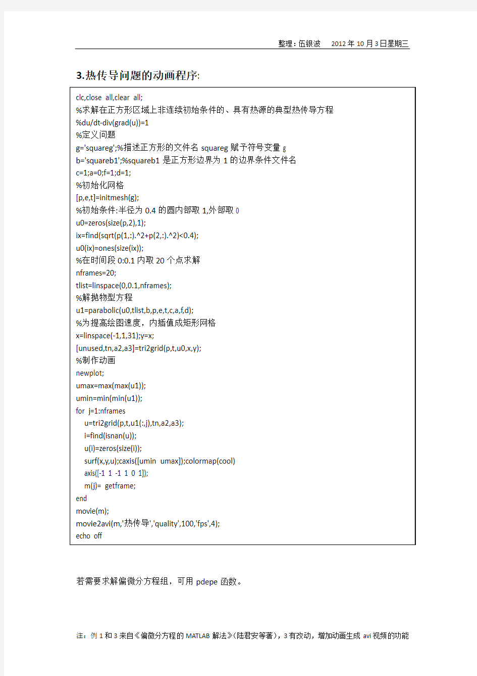
3.热传导问题的动画程序:
若需要求解偏微分方程组,可用pdepe函数。
4.非均质板壁的一维不稳定导热过程:
可用parabolic 函数求解,该函数的说明如下
:
类比可得系数c=1,a=0,f=0,d=1.计算参考程序如下:
[p,e,t]=initmesh('squareg');
[p,e,t]=refinemesh('squareg',p,e,t);
u0=zeros(size(p,2),1);
ix=find(sqrt(p(1,:).^2+p(2,:).^2)<0.8);
u0(ix)=ones(size(ix));
tlist=linspace(0,0.1,20);
u1=parabolic(u0,tlist,'squareb1',p,e,t,1,0,0,1);
pdeplot(p,e,t,'xydata',u1(:,8),'mesh','off','colormap','hot');
x=linspace(-1,1,31);y=x;
[unused,tn,a2,a3]=tri2grid(p,t,u0,x,y);
%制作动画
newplot;
umax=max(max(u1));
umin=min(min(u1));
for j=1:8
u=tri2grid(p,t,u1(:,j),tn,a2,a3);
i=find(isnan(u));
u(i)=zeros(size(i));
surf(x,y,u);caxis([umin umax]);colormap(hot)
axis([-1 1 -1 1 0 1]);
m(j)= getframe;
end movie(m);
x
t x x a x t x a t ??????τ??)()(22+=
MATLAB编辑一维热传导方程的模拟程序
求解下列热传导问题: ()()()()?????????====-=≤≤=??-??1, 10,,1,010,001222ααL t L T t T z z T L z t T z T 程序: function heat_conduction() %一维齐次热传导方程 options={'空间杆长L','空间点数N' ,'时间点数M','扩散系数alfa','稳定条件的值lambda(取值必须小于',}; topic='seting'; lines=1; ; def={'1','100','1000','1',''}; h=inputdlg(options,topic,lines,def); L=eval(h{1}); N=eval(h{2}); M=eval(h{3}); alfa=eval(h{4}); lambda=eval(h{5});%lambda 的值必须小于 %*************************************************** ¥ h=L/N;%空间步长 z=0:h:L; z=z'; tao=lambda*h^2/alfa;%时间步长 tm=M*tao;%热传导的总时间tm t=0:tao:tm; t=t'; %计算初值和边值 @ T=zeros(N+1,M+1); Ti=init_fun(z); To=border_funo(t); Te=border_fune(t); T(:,1)=Ti; T(1,:)=To; T(N+1,:)=Te; %用差分法求出温度T 与杆长L 、时间t 的关系 : for k=1:M m=2;
一维热传导MATLAB模拟
昆明学院2015届毕业设计(论文) 设计(论文)题目 一维热传导问题的数值解法及其MATLAB模拟子课题题目无 姓名伍有超 学号 5 所属系物理科学与技术系 专业年级2011级物理学2班 指导教师王荣丽 2015 年 5 月
摘要 本文介绍了利用分离变量法和有限差分法来求解一维传导问题的基本解,并对其物理意义进行了讨论。从基本解可以看出,在温度平衡过程中,杠上各点均受初始状态的影响,而且基本解也满足归一化条件,表示在热传导过程中杆的总热量保持不变。通过对一维杆热传导的分析,利用分离变量法和有限差分法对一维热传导进行求解,并用MATLAB 数学软件来对两种方法下的热传导过程进行模拟,通过对模拟所得三维图像进行取值分析,得出由分离变量法和有限差分法绘制的三维图基本相同,且均符合热传导过程中温度随时间、空间的变化规律,所以两种方法均可用来解决一维热传导过程中的温度变化问题。 关键词:一维热传导;分离变量法;有限差分法;数值计算;MATLAB 模拟
Abstract In this paper, the method of variable separation and finite difference method are introduced to solve the problem of one-dimensional heat conduction problems, and the physical significance of numerical methods for heat conduction problems are discussed. From the basic solution, we can see the temperature on the bar are affected by the initial state during the process of temperature balance, and basic solution also satisfy the normalization condition which implied the invariance of the total heat in the bar during the heat conduction process. Through the analysis of the one-dimensional heat conduction, by taking use of variable separation method and finite difference method, we simulated the one-dimensional heat conduction problem by MATLAB. The three-dimensional images of the simulation results obtained by the method of separation of variables and finite difference method are similar to each other, and the temperature curve is in accordance with the law of temperature variation during heat conduction. Thus, we can go to the conclusion that both methods can be used to deal with the one-dimensional heat conduction problems. Keywords: One-dimensional heat conduction; method of variable separation; finite difference method; numerical method; MATLAB simulation
导热方程求解matlab
使用差分方法求解下面的热传导方程 2 (,)4(,) 0100.2t xx T x t T x t x t =<<<< 初值条件:2(,0)44T x x x =- 边值条件:(0,)0(1,)0 T t T t == 使用差分公式 1,,1,2 2 2 (,)2(,)(,) 2(,)()i j i j i j i j i j i j xx i j T x h t T x t T x h t T T T T x t O h h h -+--++-+= +≈ ,1,(,)(,) (,)()i j i j i j i j t i j T x t k T x t T T T x t O k k k ++--= +≈ 上面两式带入原热传导方程 ,1,1,,1,2 2i j i j i j i j i j T T T T T k h +-+--+= 令2 24k r h =,化简上式的 ,1,1,1,(12)()i j i j i j i j T r T r T T +-+=-++ i x j t j
编程MA TLAB 程序,运行结果如下 1 x t T function mypdesolution c=1; xspan=[0 1]; tspan=[0 0.2]; ngrid=[100 10]; f=@(x)4*x-4*x.^2; g1=@(t)0; g2=@(t)0; [T,x,t]=rechuandao(c,f,g1,g2,xspan,tspan,ngrid); [x,t]=meshgrid(x,t); mesh(x,t,T); xlabel('x') ylabel('t') zlabel('T') function [U,x,t]=rechuandao(c,f,g1,g2,xspan,tspan,ngrid) % 热传导方程:
Matlab解热传导方程代码
Sample MATLAB codes 1. %Newton Cooling Law clear; close all; clc; h = 1; T(1) = 10; %T(0) error = 1; TOL = 1e-6; k = 0; dt = 1/10; while error > TOL, k = k+1; T(k+1) = h*(1-T(k))*dt+T(k); error = abs(T(k+1)-T(k)); end t = linspace(0,dt*(k+1),k+1); plot(t,T),hold on, plot(t,1,'r-.') xlabel('Time'),ylabel('Temperature'), title(['T_0 = ',num2str(T(1)), ', T_\infty = 1']), legend('Cooling Trend','Steady State') 2. %Boltzman Cooling Law clear; close all; clc; h = 1; T(1) = 10; %T(0) error = 1; TOL = 1e-6; k = 0; dt = 1/10000; while error > TOL, k = k+1; T(k+1) = h*(1-(T(k))^4)*dt+T(k); error = abs(T(k+1)-T(k)); end t = linspace(0,dt*(k+1),k+1); plot(t,T),hold on, plot(t,1,'r-.') xlabel('Time'),ylabel('Temperature'), title(['T_0 = ',num2str(T(1)), ', T_\infty = 1']), legend('Cooling Trend','Steady State') 3. %Fourier Heat conduction clear; close all; clc; h = 1; n = 11; T = ones(n,1); Told = T; T(1) = 1; %Left boundary T(n) = 10; %Right boundary x = linspace(0,1,n); dx = x(2)-x(1);
MATLAB编辑一维热传导方程的模拟程序
求解下列热传导问题: 2T 1 T 门 c , 2 0 0 z L z t T乙0 1 z2 T 0,t 1, T L,t 0 L 1, 1 程序: fun ctio n heat_c on ductio n() % 一维齐次热传导方程 options={'空间杆长L','空间点数N','时间点数M','扩散系数alfa',' 件的值 稳定条lambda(取值必须小于0.5)',}; topic='set in g'; lin es=1; def={'1','100','1000','1','0.5'}; h=in putdlg(opti on s,topic, lin es,def); L=eval(h{1}); N=eval(h{2}); M=eval(h{3}); alfa=eval(h{4}); lambda=eval(h{5});%lambda 的值必须小于0.5 o%*************************************************** h=L/N;%空间步长 z=0:h:L; z=z'; tao=lambda*h A2/alfa;% 时间步长 tm=M*tao;%热传导的总时间tm t=0:tao:tm; t=t'; %计算初值和边值 T=zeros(N+1,M+1); Ti=i nit_fu n(z); To=border_fu no (t); Te=border_fu ne(t); T(:,1)=Ti;- T(1,:)=To; T(N+1,:)=Te; %用差分法求出温度T与杆长L、时间t的关系 for k=1:M m=2; while m<=N T(m,k+1)=lambda*(T(m+1,k)+T(m-1,k))+(-2*lambda+1)*T(m,k); m=m+1; end;
热传导方程的求解
应用物理软件训练 前言 MATLAB 是美国MathWorks公司出品的商业数学软件,用于算法开发、数据可视化、数据分析以及数值计算的高级技术计算语言和交互式环境,主要包括MATLAB和Simulink两大部分。 MATLAB是矩阵实验室(Matrix Laboratory)的简称,和Mathematica、Maple 并称为三大数学软件。它在数学类科技应用软件中在数值计算方面首屈一指。MATLAB可以进行矩阵运算、绘制函数和数据、实现算法、创建用户界面、连接其
他编程语言的程序等,主要应用于工程计算、控制设计、信号处理与通讯、图像处理、信号检测、金融建模设计与分析等领域。本部分主要介绍如何根据所学热传导方程的理论知识进行MATLAB数值实现可视化。本部分主要介绍如何根据所学热传导方程的理论知识进行MATLAB数值实现可视化。本部分主要介绍如何根据所学热传导方程的理论知识进行MATLAB数值实现可视化。 本部分主要介绍如何根据所学热传导方程的理论知识进行MATLAB数值实现可视化。
题目:热传导方程的求解 目录 一、参数说明 (1) 二、基本原理 (1) 三、MATLAB程序流程图 (3) 四、源程序 (3) 五、程序调试情况 (6) 六、仿真中遇到的问题 (9) 七、结束语 (9) 八、参考文献 (10)
一、参数说明 U=zeros(21,101) 返回一个21*101的零矩阵 x=linspace(0,1,100);将变量设成列向量 meshz(u)绘制矩阵打的三维图 axis([0 21 0 1]);横坐标从0到21,纵坐标从0到1 eps是MATLAB默认的最小浮点数精度 [X,Y]=pol2cart(R,TH);效果和上一句相同 waterfall(RR,TT,wn)瀑布图 二、基本原理 1、一维热传导问题 (1)无限长细杆的热传导定解问题 利用傅里叶变换求得问题的解是: 取得初始温度分布如下 这是在区间0到1之间的高度为1的一个矩形脉冲,于是得 (2)有限长细杆的热传导定解问题
matlab求解热传导实例
matlab 求解热传导问题的几个例子 1.金属板导热问题 解: 2.Matlab 自带例子 :
3.热传导问题的动画程序: 若需要求解偏微分方程组,可用pdepe函数。
4.非均质板壁的一维不稳定导热过程: 可用parabolic 函数求解,该函数的说明如下 : 类比可得系数c=1,a=0,f=0,d=1.计算参考程序如下: [p,e,t]=initmesh('squareg'); [p,e,t]=refinemesh('squareg',p,e,t); u0=zeros(size(p,2),1); ix=find(sqrt(p(1,:).^2+p(2,:).^2)<0.8); u0(ix)=ones(size(ix)); tlist=linspace(0,0.1,20); u1=parabolic(u0,tlist,'squareb1',p,e,t,1,0,0,1); pdeplot(p,e,t,'xydata',u1(:,8),'mesh','off','colormap','hot'); x=linspace(-1,1,31);y=x; [unused,tn,a2,a3]=tri2grid(p,t,u0,x,y); %制作动画 newplot; umax=max(max(u1)); umin=min(min(u1)); for j=1:8 u=tri2grid(p,t,u1(:,j),tn,a2,a3); i=find(isnan(u)); u(i)=zeros(size(i)); surf(x,y,u);caxis([umin umax]);colormap(hot) axis([-1 1 -1 1 0 1]); m(j)= getframe; end movie(m); x t x x a x t x a t ??????τ??)()(22+=
一维热传导MATLAB模拟
一维热传导MATLAB模拟 昆明学院2015 届毕业设计设计题目一维热传导问题的数值解法及其MATLAB模拟子课题题目无姓名伍有超学号201117030225所属系物理科学与技术系专业年级2011级物理学2班指导教师王荣丽2015 年 5 月一维热传导问题的数值解法及MATLAB模拟摘要介绍了利用分离变量法和有限差分法来求解一维传导问题的基本解,并对其物理意义进行了讨论。从基本解可以看出,在温度平衡过程中,杠上各点均受初始状态的影响,而且基本解也满足归一化条件,表示在热传导过程中杆的总热量保持不变。通过对一维杆热传导的分析,利用分离变量法和有限差分法对一维热传导进行求解,并用
MATLAB 数学软件来对两种方法下的热传导过程进行模拟,通过对模拟所得三维图像进行取值分析,得出分离变量法和有限差分法绘制的三维图基本相同,且均符合热传导过程中温度随时间、空间的变化规律,所以两种方法均可用来解决一维热传导过程中的温度变化问题。关键词:一维热传导;分离变量法;有限差分法;数值计算;MATLAB 模拟 1 一维热传导问题的数值解法及MATLAB 模拟Abstract In this paper, the method of variable separation and finite difference method are introduced to solve the problem of one-dimensional heat conduction problems, and the physical significance of numerical methods for heat conduction problems are discussed. From the basic solution, we can see the temperature on the bar are affected by the initial state during the process of temperature balance, and basic solution
利用matlab程序解决热传导问题
哈佛大学能源与环境学院 课程作业报告 作业名称:传热学大作业——利用matlab程序解决热传导问题 院系:能源与环境学院 专业:建筑环境与设备工程 学号: 姓名:盖茨比 2015年6月8日
一、题目及要求 1.原始题目及要求 2.各节点的离散化的代数方程 3.源程序 4.不同初值时的收敛快慢 5.上下边界的热流量(λ=1W/(m℃)) 6.计算结果的等温线图 7.计算小结 题目:已知条件如下图所示: 二、各节点的离散化的代数方程 各温度节点的代数方程 ta=(300+b+e)/4 ; tb=(200+a+c+f)/4; tc=(200+b+d+g)/4; td=(2*c+200+h)/4 te=(100+a+f+i)/4; tf=(b+e+g+j)/4; tg=(c+f+h+k)/4 ; th=(2*g+d+l)/4 ti=(100+e+m+j)/4; tj=(f+i+k+n)/4; tk=(g+j+l+o)/4; tl=(2*k+h+q)/4
tm=(2*i+300+n)/24; tn=(2*j+m+p+200)/24; to=(2*k+p+n+200)/24; tp=(l+o+100)/12 三、源程序 【G-S迭代程序】 【方法一】 函数文件为: function [y,n]=gauseidel(A,b,x0,eps) D=diag(diag(A)); L=-tril(A,-1); U=-triu(A,1); G=(D-L)\U; f=(D-L)\b; y=G*x0+f; n=1; while norm(y-x0)>=eps x0=y; y=G*x0+f; n=n+1; end 命令文件为: A=[4,-1,0,0,-1,0,0,0,0,0,0,0,0,0,0,0; -1,4,-1,0,0,-1,0,0,0,0,0,0,0,0,0,0; 0,-1,4,-1,0,0,-1,0,0,0,0,0,0,0,0,0;
matlab求解热传导实例(可编辑修改word版)
matlab 求解热传导问题的几个例子1.金属板导热问题 解: 2.M atlab 自带例子: [p,e,t]=initmesh('squareg'); [p,e,t]=refinemesh('squareg',p,e,t); u0=zeros(size(p,2),1); ix=find(sqrt(p(1,:).^2+p(2,:).^2)<0.4); u0(ix)=ones(size(ix)); tlist=linspace(0,0.1,20); u1=parabolic(u0,tlist,'squareb1',p,e,t,1,0,1,1); pdeplot(p,e,t,'xydata',u1(:,20),'mesh','off','colormap','hot'); [p,e,t]=initmesh('crackg'); u=parabolic(0,0:0.5:5,'crackb',p,e,t,1,0,0,1); pdeplot(p,e,t,'xydata',u(:,11),'mesh','off','colormap','hot');
3.热传导问题的动画程序: clc,close all,clear all; %求解在正方形区域上非连续初始条件的、具有热源的典型热传导方程%du/dt-div(grad(u))=1 %定义问题 g='squareg';%描述正方形的文件名squareg 赋予符号变量g b='squareb1';%squareb1 是正方形边界为1 的边界条件文件名 c=1;a=0;f=1;d=1; %初始化网格 [p,e,t]=initmesh(g); %初始条件:半径为0.4 的圆内部取1,外部取0 u0=zeros(size(p,2),1); ix=find(sqrt(p(1,:).^2+p(2,:).^2)<0.4); u0(ix)=ones(size(ix)); %在时间段0:0.1 内取20 个点求解 nframes=20; tlist=linspace(0,0.1,nframes); %解抛物型方程 u1=parabolic(u0,tlist,b,p,e,t,c,a,f,d); %为提高绘图速度,内插值成矩形网格 x=linspace(-1,1,31);y=x; [unused,tn,a2,a3]=tri2grid(p,t,u0,x,y); % 制作动画 newplot; umax=max(max(u1)); umin=min(min(u1)); for j=1:nframes u=tri2grid(p,t,u1(:,j),tn,a2,a3); i=find(isnan(u)); u(i)=zeros(size(i)); surf(x,y,u);caxis([umin umax]);colormap(cool) axis([-1 1 -1 1 0 1]); m(j)= getframe; end movie(m); movie2avi(m,'热传导','quality',100,'fps',4); echo off 若需要求解偏微分方程组,可用pdepe 函数。
(完整word版)matlab求解热传导实例
matlab求解热传导问题的几个例子1.金属板导热问题 解: 2.Matlab自带例子: [p,e,t]=initmesh('crackg'); u=parabolic(0,0:0.5:5,'crackb',p,e,t,1,0,0,1); pdeplot(p,e,t,'xydata',u(:,11),'mesh','off','colormap','hot'); [p,e,t]=initmesh('squareg'); [p,e,t]=refinemesh('squareg',p,e,t); u0=zeros(size(p,2),1); ix=find(sqrt(p(1,:).^2+p(2,:).^2)<0.4); u0(ix)=ones(size(ix)); tlist=linspace(0,0.1,20); u1=parabolic(u0,tlist,'squareb1',p,e,t,1,0,1,1); pdeplot(p,e,t,'xydata',u1(:,20),'mesh','off','colormap','hot');
3.热传导问题的动画程序: 若需要求解偏微分方程组,可用pdepe函数。
4.非均质板壁的一维不稳定导热过程:可用parabolic函数求解,该函数的说明如下: 类比可得系数c=1,a=0,f=0,d=1.计算参考程序如下: [p,e,t]=initmesh('squareg'); [p,e,t]=refinemesh('squareg',p,e,t); u0=zeros(size(p,2),1); ix=find(sqrt(p(1,:).^2+p(2,:).^2)<0.8); u0(ix)=ones(size(ix)); tlist=linspace(0,0.1,20); u1=parabolic(u0,tlist,'squareb1',p,e,t,1,0,0,1); pdeplot(p,e,t,'xydata',u1(:,8),'mesh','off','colormap','hot'); x=linspace(-1,1,31);y=x; [unused,tn,a2,a3]=tri2grid(p,t,u0,x,y); %制作动画 newplot; umax=max(max(u1)); umin=min(min(u1)); for j=1:8 u=tri2grid(p,t,u1(:,j),tn,a2,a3); i=find(isnan(u)); u(i)=zeros(size(i)); surf(x,y,u);caxis([umin umax]);colormap(hot) axis([-1 1 -1 1 0 1]); m(j)= getframe; end movie(m); x t x x a x t x a t ? ? ? ? ? ? τ ? ?) ( ) ( 2 2 + =