Maxwell仿真圆柱体电容器
电磁场与电磁波项目训练报告
仿真求解圆柱形电容器
班级:通信13-2
姓名:闫振宇
学号:1306030222
指导教师:徐维老师
成绩:
电子与信息工程学院
信息与通信工程系
项目训练一 仿真求解圆柱形电容器
1. 实验目的和任务
1)掌握用ANSYS Maxwell 软件仿真的方法;
2)学会利用所学的场强,电容,电场的知识来解决实际现实生活中的计算问题; 3)利用ANSYS Maxwell 软件仿真圆柱形电容器。
2. 实验内容
1)学习ANSYS Maxwel 有限元分析步骤; 2)学习ANSYS Maxwel 的基本仿真操作步骤;
3)对圆柱体电容器计算理论值和实验的仿真值进行比较,得出结论。
3. 实验原理
电容是反映电容器储存的电荷本领大小的物理量。
电容的定义:一个电容器所带的电量Q 总与其电压U 成正比,比值Q/U 叫电容器的电容。以C 表示电容器的电容,就有公式:
U
Q C =
电容器的电容决定于电容器的本身结构,即是导体的形状,尺寸以及两导体间电介质的种类等,而与它所带的电量无关。
首先,假设本题中圆柱体电容器的内部的外表面,和外部的内表面分别带有绝对值为Q 的电量。两筒之间充满相对介电常数为
εr
的电介质。(m F o 1012
855313.8-?=ε)
所以,在距离轴线为r 的电介质中一点的电场强度E 为:
rL
Q E r εεπ 2=
对E 进行积分,可以得到两圆筒间的电压U 为:
dr R
R rL Q U r ?=212εεπ =R R L Q r 1
2ln 2εεπ
就得到了圆柱形电容器的电容C 为:
)
ln(21
2
R
R L C r εεπ =
根据以上的公式,代入R2=1mm,R1=0.6mm,得出长度为L的圆柱形电容器电容。
4.实验步骤
4.1建模(Model)
Project > Insert Maxwell 3D Design
File>Save as>Cylinder Cap(工程命名为“Cylinder yuanzhuti”)
选择求解器类型:Maxwell > Solution Type> Electric> Electrostatic(静电的)
4.1.1 创建中心圆柱体导体
Draw > Cylinder(中心圆柱体导体)
圆柱中心点坐标:(X,Y,Z)>(0, 0, 0)mm
坐标偏置:(dX,dY,dZ)>(0.6, 0.6,0)mm
坐标偏置:(dX,dY,dZ)>(0, 0, 2)mm
将圆柱体重命名为Cylinder5
Assign Material > copper(设置材料为铜copper)
4.1.2 创建内外导体间空心圆柱体介质
Draw > Cylinder(中心圆柱体导体)
圆柱中心点坐标:(X,Y,Z)>(0, 0, 0)mm
坐标偏置:(dX,dY,dZ)>(0.6, 0.6,0)mm
坐标偏置:(dX,dY,dZ)>(0, 0, 2)mm
将圆柱体重命名为Cylinder1
Draw > Cylinder(中心圆柱体导体)
圆柱中心点坐标:(X,Y,Z)>(0, 0, 0)mm
坐标偏置:(dX,dY,dZ)>(1.0, 1.0,0)mm
坐标偏置:(dX,dY,dZ)>(0, 0, 2)mm
将圆柱体重命名为Cylinder2
选中Cylinder1,Cylinder2
Modeler (建模)> Boolean > Sbutract(分离)
Blank park:Cylinder1
Tool park:Cylinder2
将分离出的圆环命名为Cylinder4
Assign Material > air(设置材料为空气air)
4.1.3创建外空心圆柱体导体
Draw > Cylinder(中心圆柱体导体)
圆柱中心点坐标:(X,Y,Z)>(0, 0, 0)mm
坐标偏置:(dX,dY,dZ)>(1.0, 1.0,0)mm
坐标偏置:(dX,dY,dZ)>(0, 0, 2)mm
将圆柱体重命名为Cylinder6
Draw > Cylinder(中心圆柱体导体)
圆柱中心点坐标:(X,Y,Z)>(0, 0, 0)mm
坐标偏置:(dX,dY,dZ)>(1.2, 1.2,0)mm
坐标偏置:(dX,dY,dZ)>(0, 0, 2)mm
将圆柱体重命名为Cylinder7
选中Cylinder6,Cylinder7
Modeler (建模)> Boolean > Sbutract(分离)Blank park:Cylinder6
Tool park:Cylinder7
将分离出的圆环命名为Cylinder3
Assign Material > copper(设置材料为铜copper)
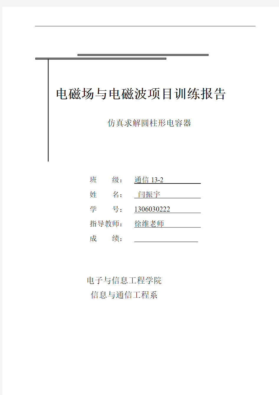
图4-1仿真效果图4.2设置参数
4.2.1 创建设置区域(Region)
Draw > Region
Padding Percentage:0%
减少电场的边缘效应(fringing effect)
4.2.2 设置激励电压(Assign Excitation)
选择Cylinder5
Maxwell 3D> Excitations > Assign>V oltage > 5V
选择Cylinder3
Maxwell 3D> Excitations > Assign >V oltage > 0V
4.2.3设置自适应计算参数(Create Analysis Setup)Maxwell 3D > Analysis Setup > Add Solution Setup
最大迭代次数:Maximum number of passes > 10
误差要求:Percent Error > 1%
每次迭代加密剖分单元比例:Refinement per Pass > 50%
4.2.4 设置计算参数(Assign Executive Parameter)Maxwell 3D > Parameters > Assign > Matrix > V oltage1, V oltage2 4.2.5 check,计算,查看结果
Maxwell 3D > Reselts > Solution data > Matrix
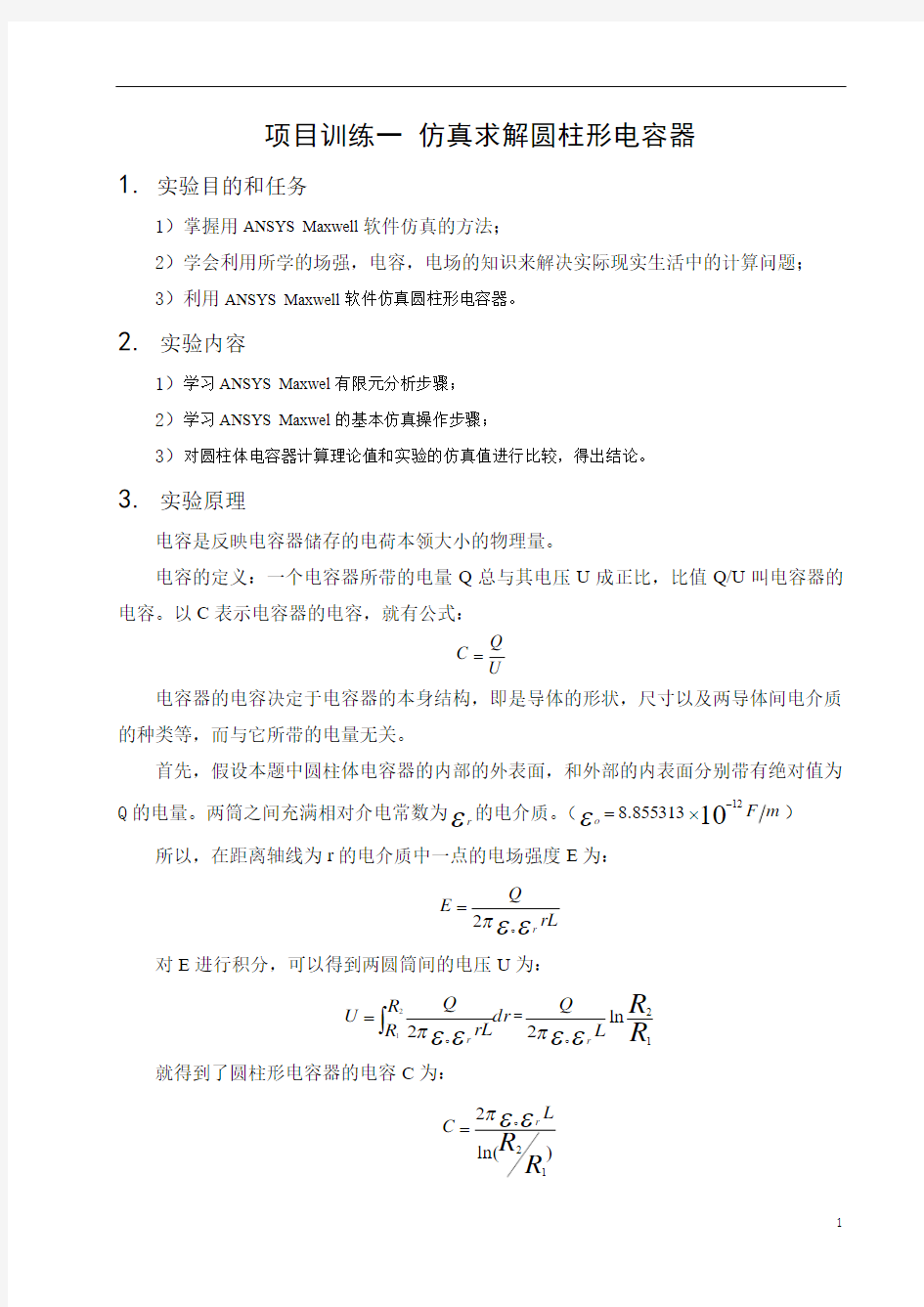
图4-2仿真数据图
5.数据
取电容器长度L为:2mm,则有:
电容值:C=0.2186pF
表 4-1 理论及仿真的值
理论计算值仿真输出值
0.2179pF 0.2186pF
图5-1电压分布图
6.心得体会
通过利用Maxwell软件制作圆柱体电容器,了解了Maxwell软件的基本操作和使用方法。了解了利用所学到的知识来解决现实生活中的实际问题,更加深入了解了学到的理论知识。在仿真的过程中,碰到了很大的问题,但是经过与同学的讨论和参考书的查阅明白了问题的所在。
Ansoft和Simplore联合仿真注意事项
1.Ansoft和Simplore联合仿真时,如果Ansoft中的模型类型是Transient,则必 须勾选Maxwell 2D -> Design Settings -> Advanced Product Coupling菜单中的Enable transient-transient link with Sim,否则在检查时会产生Cannot find the matching inductor in the imported file 这个错误。 2.Ansoft和Simplore联合仿真时,Simplore软件控制着仿真步长,也控制着 Ansoft模型的旋转速度(或者称线速度)。 3.Ansoft和Simplore联合仿真的必要前提: 1)Ansoft模型必须可以求解(即可以进行运算)。 2)Ansoft模型必须含有机械运动(原文: must have mechanical motion) 3)Ansoft模型必须至少含有一个外部类型(external类型)的绕组。 4)Ansoft模型名不能含有非法字符(如空格) 5)建议:在与Simplore联合仿真之前,最好保证Ansoft模型可以单独进行 运算(即可以Solve without external windings) 4.Ansoft和Simplore联合仿真时,Ansoft软件内部设定的开始和停止时间会发 生变化(即由Simplore控制) 5.Ansoft的仿真停止时间必须大于或等于Simplore的仿真停止时间。 6.Ansoft和Simplore联合仿真,Ansoft模型必须含有:几何图形,运动的Band (moving band),材料,边界条件,external 类型的绕组,剖分。
Maxwell与Simplorer联合仿真方法及注意问题
三相鼠笼式异步电动机的协同仿真模型实验分析 本文所采用的电机是参照《Ansoft 12在工程电磁场中的应用》一书所给的使用RMxprt输入机械参数所生成的三相鼠笼式异步电动机,并且由RMxprt的电机模型直接导出2D模型。由于个人需要,对电机的参数有一定的修改,但是使用Y160M--4的电机并不影响联合仿真的过程与结果。 1.1 Maxwell与Simplorer联合仿真的设置 1.1.1Maxwell端的设置 在Maxwell 2D模型中进行一下几步设置: 第一步,设置Maxwell和Simplorer端口连接功能。右键单击Model项,选择Set Symmetry Multiplier项,如图1.1所示,单击后弹出图1.2的对话框。 图1.1 查找过程示意图
图1.2 设计设置对话框 在对话框中,选择Advanced Product Coupling项,勾选其下的Enable tr-tr link with Sim 。至此,完成第一步操作。 第二步,2D模型的激励源设置。单击Excitation项的加号,显示Phase A、Phase B、Phase C各项。双击Phase A项,弹出如图1.3所示的对话框。 图1.3 A相激励源设置 在上图的对话框中,将激励源的Type项设置为External,并勾选其后的Strander,并且设置初始电流Initial Current项为0。Number of parallel branch项按照电机的设置要求,其值为1。参数设置完成后,点击确定退出。 需要说明的一点是,建议在设置Maxwell与Simplorer连接功能即第一步之前,记录电压激励源下的电阻和电感。事实上,这里的电组和电感就是Maxwell 2D计算出的电机的定子电阻与定子电感。这两个数据在外电路的连接中会使用到,在后面会详细说明。 至此,Maxwell端的设置完毕。 1.1.2 Simplorer端的设置 Simplorer端的设置,主要是对电机外电路的设置,具体的电路会在空载实验和额定负载实验中详细给出,这里不再赘述。
simplorer-maxwell联合仿真实例
T1T2T3T4
Co-simulation with Maxwell Technical Background The co-simulation is the most accurate way of coupling the drive and the motor model. The advantage of this method is the high accuraty, having the real inverter currents as source in Maxwell and the back emf of the motor on the inverter currents as source in Maxwell, and the back-emf of the motor on the inverter side. The transient-transient link enables the use to pass data between Simplorer and Maxwell during the simulation: Maxwell2D and Maxwell3D can be used Simplorer and Maxwell will run altogether Simplorer is the Master, Maxwell is the slave At a given time step, the Winding currents and the Rotor angle are passed from Simplorer to Maxwell, the Back EMF and the Torque are passed from Maxwell to Simplorer The complexity of the drive system and of the mechanical system is not The complexity of the drive system and of the mechanical system is not limited Insights on the coupling Method The Simplorer time steps and the Maxwell time steps don’t have to be the same. Usually, Simplorer requires much more time steps than Maxwell. Assume the current simulation time is t Simplorer, based on the previous time steps, gives a forward meeting time t1to Maxwell where both simulators will exchange data. Between t0and t1, both code run by themselves. At t 1, both codes exchange data. If during the t0-t1period, some event appears on Simplorer side (state graph transition, large change of the pp p(g p,g g dynamic of the circuit), Simplorer will roll back to t0and set a new forward meeting time t1’, t1’< t1.
sim-sim-maxwell联合仿真遇到的问题及解决方法
sim-sim-maxwell联合仿真遇到的问题及解决方法
Maxwell、Simplorer与Simulink联合仿真 [请输入文档摘要,摘要通常是对文档内容的简短总结。输入文档摘要,摘要通常 是对文档内容的简短总结。] 错误!未找到引用源。
目录 前言 (3) 一、在Maxwell里建立仿真模型,并设置联合仿真参数 (4) 二、Simplorer (7) 三、Simplorer与Maxwell的联合 (8) 三、Simplorer与Simulink (9) 1、在Simplorer里的操作 (10) 2、在Simulink里的操作 (13) 五、求解器参数的设置 (18) 常见的问题 (20) 前言
本文主要介绍Maxwell、Simplorer和Simulink如何实现联合仿真,已经出现的问题和解决方法。以直线开关磁阻电机为仿真模型,对电机模型的参数进行辨识,控制算法采用PID和极点配置自适应控制算法。用到的软件版本分别为:Maxwell 13、Simplorer 9.0和MATLAB R2007b。三个软件里建立的工程或模型文件必须放在同一个文件夹里,仿真中需要建立的和分析后生成的文件如图1所示。 图 1 在Maxwell里建立有限元仿真模型;Simplorer 提供功率电路部分,是将Maxwell和Simulink连接起来的桥梁;Simulink 为联合仿真提供控制算法,输入为期望的位置信号和实际的位置信号(从Simplorer里输入)输出为三相电流信号。 一、在Maxwell里建立仿真模型,并设置联合仿真参数 1、根据实际电机的尺寸和材料建立直线开关磁阻电机的磁场瞬态分析模型,如图2所示。
Ansoft与Workbench协同仿真实现双向耦合的方法
Ansoft与Workbench协同仿真实现双向耦合的方法在科研或者做研究生毕设的过程中,经常会遇到多个物理场的耦合问题,诸如流固耦合、热电耦合、磁热耦合以及磁热结构耦合等等。而且往往还会遇到各种非线性问题:磁导率是随温度变化的或者电阻率也与温度成非线性关系,这时为了保证计算结果的准确性,有必要也必须是多物理场实现双向耦合。 在Ansoft与Workbench实现磁热耦合的过程中,就需要保证他们耦合式双向的。下面介绍两种方法: 方案一:利用Workbench组件系统中的“Feedback Iterator”模块,如下图 然后设置Feedback Iterator属性,也可添加脚本。 使用这种方法,通常3-4次耦合迭代即可达到稳定(Ansys官方说法)
方案二:Ansoft Help文档—“Coupling Maxwell Designs with ANSYS Thermal via Workbench” 19. To export the thermal result to Maxwell, right-click on the Imported Load (Maxwell2DSolution), or Imported Load(Maxwell3DSolution) and select Export Results. 20. To fully utilize the automation capabilities provided in ANSYS Workbench, select Imported Load (Maxwell2DSolution), or Imported Load(Maxwell3DSolution); and in its Detail window, select Yes for Export after Solve. With this option selected, users can continue the iteration between Maxwell/Thermal simulations from the Workbench schematic. To “push” the exported thermal results back to Maxwell, right-click on Maxwell's Solution cell on the Workbench schematic and select Enable Update. Then, right-click again on Maxwell's Solution cell and select Update. This will trigger Maxwell to re-simulate its solution with thermal results. To continue the solve iterations, repeat the following steps as needed: a. Right-click on Thermal's Setup cell and select Refresh. b. Right-click on Thermal's Setup cell and select Update. c. Right-click on Maxwell's Solution cell and select Enable Update. d. Right-click on Maxwell's Solution cell and select Updat e.
maxwell和workbench的联合仿真
Coupling Maxwell Designs with ANSYS Thermal via Workbench Coupling Maxwell2D/3D V15 with ANSYS R14 is supported via the Workbench schematic. Thermal feedback is supported for Maxwell magnetostatic, eddy current, and transient types. Users also need to setup the design and geometry appropriately. An appropriate design should be temperature-dependent, and have one or more solve setups that are enabled for thermal feedback. 1. The easiest way to add a Maxwell 2D or 3D design to a Workbench schematic is to import a working design via Workbench File>Import. The imported design is placed in the Workbench schematic after it is successfully imported. 2. Next, insert a Steady-State Thermal system and change its Analysis Type to 2D or 3D, (depending on the Maxwell design type) by right clicking on the Geometry cell and selecting Properties. It is important to change the Steady-State Thermal system's analysis type before setting up its geometry. 3. To setup the Steady-State Thermal system's geometry, you must first export the Maxwell geometry using sat or step format as follows: a. Select the Modeler>Export menu item. b. Select the desired model geometry format (sat or step), and the save location in the dialog box and save the file for use by ANSYS Workbench. 4. Import the file via the Geometry module of the Steady-State Thermal system.
RMXPRT&maxwell&simplorer联合仿真——实例
题目: RMXPRT / MAXWELL和SIMPLORER的联合仿真 作者: ENZO 软件:MAXWELL 11.1.1 , SIMPLORER 7.05 1. 建立RMXPRT模型 电机为4极9槽稀土永磁无刷电机,这里不讨论电机的实际设计,所以具体参数不列出了,只当作操作步骤演示。 2. 设置好电机的各项参数后,计算电机的性能,得到电机的特性参数,后面将对RMXPRT 的数据和SIMPLORER的数据做比较,所以这里列出了电机的力矩和电流曲线。 力矩-转速曲线
电流-转速曲线 请注意6000RPM时的力矩和电流数值,分别为124mNm , 4.18A. 请注意在这个例子里设置了限流值5.0A ,后面SIMPLORER里同样有这个设置。 3. 输出RMXPRT的SIMPLORER模型,步骤见下图 4. 到这里RMXPRT的操作就结束了,输出的模型A相绕组的中心对准磁极的中心. 这个很重要,在RMXPRT中,对准是自动进行的,在MAXWELL里就要使用者自己来做。 5. 在SIMPLORER中导入前面建立的RMXPRT模型,
6. 将上图中的RMX-LINK图标拖到SIMPLORER SCHEMATIC的窗口中,双击图标 电机IMPORT MODEL, 在路径中指定RMXPRT 的SIMPLORER模型的路径,这样,电机的SIMPLORER 模型就导入了, RMX-LINK图标变成了电机的实际外形。下面是逆变器模型。 7. 逆变器用MOSFET构成,这里为了简化, MOSFET用了系统级的元件模型。
8. MOSFET 驱动电路
sim_sim maxwell联合仿真遇到的问题及解决方法
Maxwell、Simplorer与Simulink联合仿真 [请输入文档摘要,摘要通常是对文档内容的简短总结。输入文档摘要,摘要通常 是对文档内容的简短总结。] 错误!未找到引用源。
目录 前言 (2) 一、在Maxwell里建立仿真模型,并设置联合仿真参数 (3) 二、Simplorer (6) 三、Simplorer与Maxwell的联合 (7) 三、Simplorer与Simulink (8) 1、在Simplorer里的操作 (9) 2、在Simulink里的操作 (12) 五、求解器参数的设置 (16) 常见的问题 (18) 前言
本文主要介绍Maxwell、Simplorer和Simulink如何实现联合仿真,已经出现的问题和解决方法。以直线开关磁阻电机为仿真模型,对电机模型的参数进行辨识,控制算法采用PID和极点配置自适应控制算法。用到的软件版本分别为:Maxwell 13、Simplorer 9.0和MATLAB R2007b。三个软件里建立的工程或模型文件必须放在同一个文件夹里,仿真中需要建立的和分析后生成的文件如图1所示。 图 1 在Maxwell里建立有限元仿真模型;Simplorer 提供功率电路部分,是将Maxwell和Simulink连接起来的桥梁;Simulink 为联合仿真提供控制算法,输入为期望的位置信号和实际的位置信号(从Simplorer里输入)输出为三相电流信号。 一、在Maxwell里建立仿真模型,并设置联合仿真参数 1、根据实际电机的尺寸和材料建立直线开关磁阻电机的磁场瞬态分析模型,如图2所示。
图 2 2、对电磁瞬态分析的一些仿真参数进行设置(如图3所示)。包括运动区域,求解边界条件,激励,力矩,网格剖分(理论上说网格剖分越细求解越精确,但是剖分越细求解时间越长,所以可以根据实际情况综合考虑)、分析设置(后面会讲到)。 图 3 3、联合仿真中激励的添加:激励类型选择“External”,初始值为0A,如图4所示。