Fixed-Point Filter Design

On this page…

Overview of Fixed-Point Filters

Data Types for Filter Functions

Convert a Filter from Floating Point to Fixed Point in MATLAB

Create an FIR Filter Using Integer Coefficients

Fixed-Point Filtering in Simulink

Overview of Fixed-Point Filters

The most common use of fixed-point filters is in the DSP chips, where the data storage capabilities are limited, or embedded systems and devices where low-power consumption is necessary. For example, the data input may come from a 12 bit ADC, the data bus may be 16 bit, and the multiplier may have 24 bits. Within these space constraints, DSP System Toolbox software enables you to design the best possible fixed-point filter.

What Is a Fixed-Point Filter?

lA fixed-point filter uses fixed-point arithmetic and is represented by an equation with fixed-point coefficients. To learn about fixed-point math, see Fixed-Point Concepts in Fixed-Point Toolbox documentation.

Data Types for Filter Functions

Data Type Support

Fixed Data Type Support

Single Data Type Support

Data Type Support

There are three different data types supported in DSP System Toolbox software:

Fixed — Requires Fixed Point Toolbox and is supported by packages listed in Fixed Data Type Support.

Double — Double precision, floating point and is the default data type for DSP System Toolbox software; accepted by all functions

Single — Single precision, floating point and is supported by specific packages outlined in Single Data Type Support.

Fixed Data Type Support

To use fixed data type, you must have Fixed Point Toolbox. Type ver at the MATLAB command prompt to get a listing of all installed products.

The fixed data type is reserved for any filter whose property arithmetic is set to fixed. Furthermore all functions that work with this filter, whether in analysis or design, also accept and support the fixed data types.

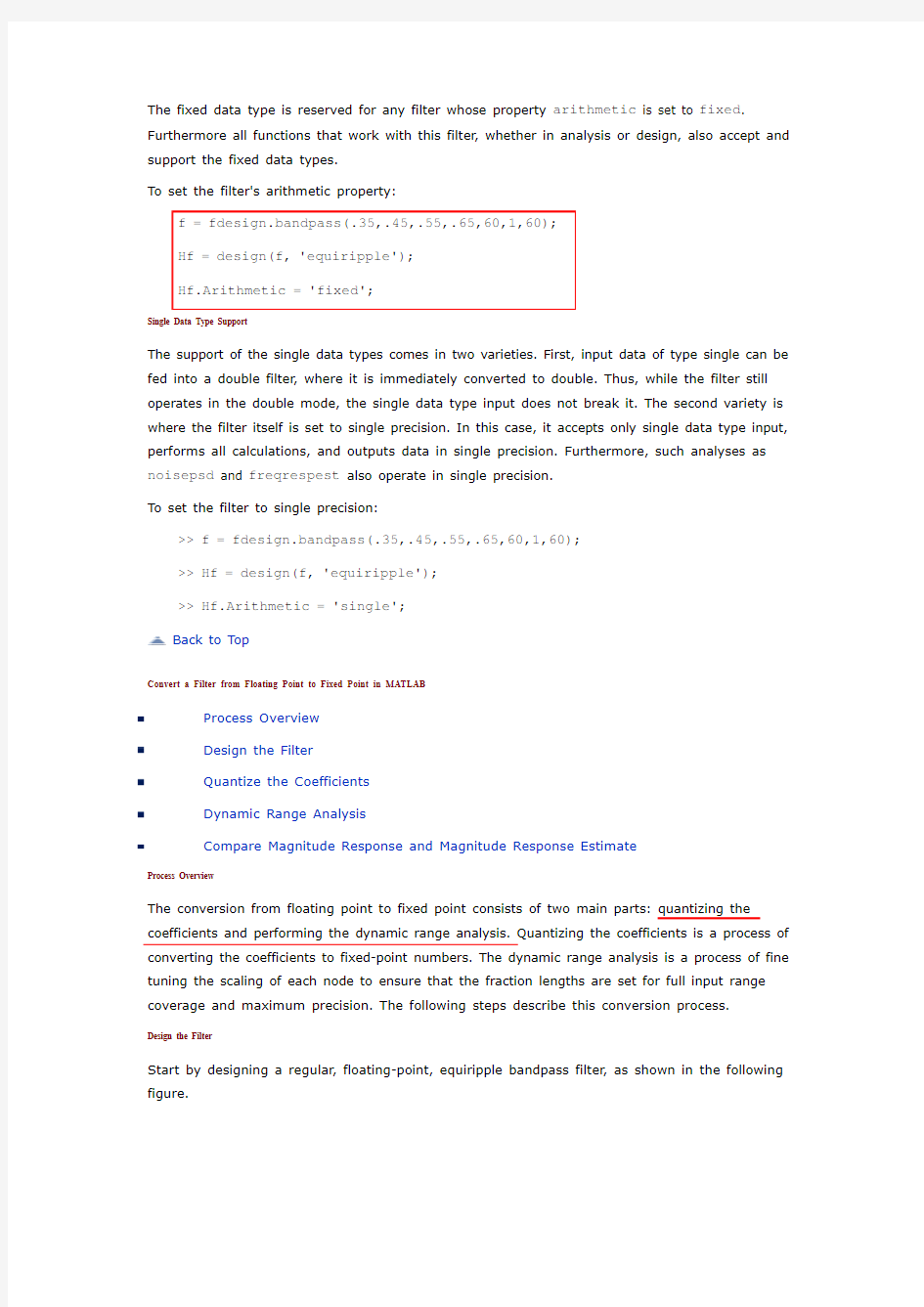
To set the filter's arithmetic property:

>> f = fdesign.bandpass(.35,.45,.55,.65,60,1,60);

>> Hf = design(f, 'equiripple');

>> Hf.Arithmetic = 'single';

Convert a Filter from Floating Point to Fixed Point in MATLAB

Process Overview

Design the Filter

Quantize the Coefficients

Dynamic Range Analysis

Compare Magnitude Response and Magnitude Response Estimate

where the passband is from .45 to .55 of normalized frequency, the amount of ripple acceptable in the passband is 1 dB, the first stopband is from 0 to .35 (normalized), the second stopband is from .65 to 1 (normalized), and both stopbands provide 60 dB of attenuation.

To design this filter, evaluate the following code, or type it at the MATLAB command prompt:

f = fdesign.bandpass(.35,.45,.55,.65,60,1,60);

Hd = design(f, 'equiripple');

fvtool(Hd)

The last line of code invokes the Filter Visualization Tool, which displays the designed filter. You use Hd, which is a double, floating-point filter, both as the baseline and a starting point for the conversion.

Quantize the Coefficients

The first step in quantizing the coefficients is to find the valid word length for the coefficients. Here again, the hardware usually dictates the maximum allowable setting. However, if this constraint is large enough, there is room for some trial and error. Start with the coefficient word length of 8 and determine if the resulting filter is sufficient for your needs.

To set the coefficient word length of 8, evaluate or type the following code at the MATLAB command prompt:

Hf = Hd;

Hf.Arithmetic = 'fixed';

set(Hf, 'CoeffWordLength', 8);

fvtool(Hf)

The resulting filter is shown in the following figure.

As the figure shows, the filter design constraints are not met. The attenuation is not complete, and there is noise at the edges of the stopbands. You can experiment with different coefficient word lengths if you like. For this example, however, the word length of 12 is sufficient.

To set the coefficient word length of 12, evaluate or type the following code at the MATLAB command prompt:

set(Hf, 'CoeffWordLength', 12);

fvtool(Hf)

The resulting filter satisfies the design constraints, as shown in the following figure.

Now that the coefficient word length is set, there are other data width constraints that might

require attention. Type the following at the MATLAB command prompt:

>> info(Hf)

Discrete-Time FIR Filter (real)

-------------------------------

Filter Structure : Direct-Form FIR

Filter Length : 48

Stable : Yes

Linear Phase : Yes (Type 2)

Arithmetic : fixed

Numerator : s12,14 -> [-1.250000e-001 1.250000e-001)

Input : s16,15 -> [-1 1)

Filter Internals : Full Precision

Output : s31,29 -> [-2 2) (auto determined)

Product : s27,29 -> [-1.250000e-001 1.250000e-001)...

(auto determined)

Accumulator : s31,29 -> [-2 2) (auto determined)

Round Mode : No rounding

Overflow Mode : No overflow

You see the output is 31 bits, the accumulator requires 31 bits and the multiplier requires 27 bits.

A typical piece of hardware might have a 16 bit data bus, a 24 bit multiplier, and an accumulator with 4 guard bits. Another reasonable assumption is that the data comes from a 12 bit ADC. To reflect these constraints type or evaluate the following code:

set (Hf, 'InputWordLength', 12);

set (Hf, 'FilterInternals', 'SpecifyPrecision');

set (Hf, 'ProductWordLength', 24);

set (Hf, 'AccumWordLength', 28);

set (Hf, 'OutputWordLength', 16);

Although the filter is basically done, if you try to filter some data with it at this stage, you may get erroneous results due to overflows. Such overflows occur because you have defined the constraints,

but you have not tuned the filter coefficients to handle properly the range of input data where the filter is designed to operate. Next, the dynamic range analysis is necessary to ensure no overflows.

Dynamic Range Analysis

The purpose of the dynamic range analysis is to fine tune the scaling of the coefficients. The ideal set of coefficients is valid for the full range of input data, while the fraction lengths maximize precision. Consider carefully the range of input data to use for this step. If you provide data that covers the largest dynamic range in the filter, the resulting scaling is more conservative, and some precision is lost. If you provide data that covers a very narrow input range, the precision can be much greater, but an input out of the design range may produce an overflow. In this example, you use the worst-case input signal, covering a full dynamic range, in order to ensure that no overflow ever occurs. This worst-case input signal is a scaled version of the sign of the flipped impulse response.

To scale the coefficients based on the full dynamic range, type or evaluate the following code:

x = 1.9*sign(fliplr(impz(Hf)));

Hf = autoscale(Hf, x);

To check that the coefficients are in range (no overflows) and have maximum possible precision, type or evaluate the following code:

fipref('LoggingMode', 'on', 'DataTypeOverride', 'ForceOff');

y = filter(Hf, x);

fipref('LoggingMode', 'off');

R = qreport(Hf)

Where R is shown in the following figure:

The report shows no overflows, and all data falls within the designed range. The conversion has completed successfully.

Compare Magnitude Response and Magnitude Response Estimate

You can use the fvtool GUI to analysis on your quantized filter, to see the effects of the quantization on stopband attenuation, etc. Two important last checks when analyzing a quantized filter are the Magnitude Response Estimate and the Round-off Noise Power Spectrum. The value of the Magnitude Response Estimate analysis can be seen in the following example.

View the Magnitude Response Estimate

Begin by designing a simple lowpass filter using the command.

h = design(fdesign.lowpass, 'butter','SOSScaleNorm','Linf');

Now set the arithmetic to fixed-point.

h.arithmetic = 'fixed';

Open the filter using fvtool.

fvtool(h)

When fvtool displays the filter using the Magnitude response view, the quantized filter seems to match the original filter quite well.

However if you look at the Magnitude Response Estimate plot from the Analysis menu, you will see that the actual filter created may not perform nearly as well as indicated by the Magnitude Response plot.

This is because by using the noise-based method of the Magnitude Response Estimate , you estimate the complex frequency response for your filter as determined by applying a noise- like signal to the filter input. Magnitude Response Estimate uses the Monte Carlo trials to generate a noise signal that contains complete frequency content across the range 0 to Fs. For more

information about analyzing filters in this way, refer to the section titled Analyzing Filters with a Noise-Based Method in the User Guide.

For more information, refer to McClellan, et al., Computer-Based Exercises for Signal Processing Using MATLAB 5, Prentice-Hall, 1998. See Project 5: Quantization Noise in Digital Filters, page 231. Back to Top

Create an FIR Filter Using Integer Coefficients

Review of Fixed-Point Numbers

Terminology of Fixed-Point Numbers. DSP System Toolbox functions assume fixed-point quantities are represented in two's complement format, and are described using the WordLength and FracLength parameters. It is common to represent fractional quantities of WordLength 16 with the leftmost bit representing the sign and the remaining bits representing the fraction to the right of the binary point. Often the FracLength is thought of as the number of bits to the right of the binary point. However, there is a problem with this interpretation when the FracLength is larger than the WordLength, or when the FracLength is negative.

To work around these cases, you can use the following interpretation of a fixed-point quantity:

The register has a WordLength of B , or in other words it has B bits. The bits are numbered from left to right from 0 to B -1. The most significant bit (MSB) is the leftmost bit, b B-1. The least significant

bit is the right-most bit, b

. You can think of the FracLength as a quantity specifying how to

interpret the bits stored and resolve the value they represent. The value represented by the bits is determined by assigning a weight to each bit:

In this figure, L is the integer FracLength. It can assume any value, depending on the quantization step size. L is necessary to interpret the value that the bits represent. This value is given by the equation

The value 2–L is the smallest possible difference between two numbers represented in this format, otherwise known as the quantization step. In this way, it is preferable to think of the FracLength as the negative of the exponent used to weigh the right-most, or least-significant, bit of the

fixed-point number.

To reduce the number of bits used to represent a given quantity, you can discard the

least-significant bits. This method minimizes the quantization error since the bits you are removing carry the least weight. For instance, the following figure illustrates reducing the number of bits from 4 to 2:

This means that the FracLength has changed from L to L – 2.

You can think of integers as being represented with a FracLength of L = 0, so that the quantization step becomes .

Suppose B = 16 and L = 0. Then the numbers that can be represented are the integers

If you need to quantize these numbers to use only 8 bits to represent them, you will want to discard the LSBs as mentioned above, so that B=8 and L = 0–8 = –8. The increments, or quantization step

then becomes . So you will still have the same range of values, but with less

precision, and the numbers that can be represented become

With this quantization the largest possible error becomes about 256/2 when rounding to the nearest, with a special case for 32767.

Integers and Fixed-Point Filters

This section provides an example of how you can create a filter with integer coefficients. In this example, a raised-cosine filter with floating-point coefficients is created, and the filter coefficients are then converted to integers.

Define the Filter Coefficients. To illustrate the concepts of using integers with fixed-point filters, this example will use a raised-cosine filter:

b = firrcos(100, .25, .25, 2, 'rolloff', 'sqrt');

The coefficients of b are normalized so that the passband gain is equal to 1, and are all smaller than 1. In order to make them integers, they will need to be scaled. If you wanted to scale them to use 18 bits for each coefficient, the range of possible values for the coefficients becomes:

Because the largest coefficient of b is positive, it will need to be scaled as close as possible to 131071 (without overflowing) in order to minimize quantization error. You can determine the exponent of the scale factor by executing:

B = 18; % Number of bits

L = floor(log2((2^(B-1)-1)/max(b))); % Round towards zero to avoid overflow bsc = b*2^L;

Alternatively, you can use the fixed-point numbers autoscaling tool as follows:

bq = fi(b, true, B); % signed = true, B = 18 bits

L = bq.FractionLength;

It is a coincidence that B and L are both 18 in this case, because of the value of the largest coefficient of b. If, for example, the maximum value of b were 0.124, L would be 20 while B (the number of bits) would remain 18.

Build the FIR Filter. First create the filter using the direct form, tapped delay line structure:

h = dfilt.dffir(bsc);

In order to set the required parameters, the arithmetic must be set to fixed-point:

h.Arithmetic = 'fixed';

h.CoeffWordLength = 18;

You can check that the coefficients of h are all integers:

all(h.Numerator == round(h.Numerator))

ans =

Now you can examine the magnitude response of the filter using fvtool:

fvtool(h, 'Color', 'white')

This shows a large gain of 108 dB in the passband, which is due to the large values of the coefficients— this will cause the output of the filter to be much larger than the input. A method of addressing this will be discussed in the following sections.

Set the Filter Parameters to Work with Integers. You will need to set the input parameters of your filter to appropriate values for working with integers. For example, if the input to the filter is from a A/D converter with 12 bit resolution, you should set the input as follows:

h.InputWordLength = 12;

h.InputFracLength = 0;

The info method returns a summary of the filter settings.

info(h)

Discrete-Time FIR Filter (real)

-------------------------------

Filter Structure : Direct-Form FIR

Filter Length : 101

Stable : Yes

Linear Phase : Yes (Type 1)

Arithmetic : fixed

Numerator : s18,0 -> [-131072 131072)

Input : s12,0 -> [-2048 2048)

Filter Internals : Full Precision

Output : s31,0 -> [-1073741824 1073741824) (auto determined) Product : s29,0 -> [-268435456 268435456) (auto determined) Accumulator : s31,0 -> [-1073741824 1073741824) (auto determined) Round Mode : No rounding

Overflow Mode : No overflow

Filter the Test Signal. To filter the input signal generated above, enter the following:

Here ysc is a full precision output, meaning that no bits have been discarded in the computation. This makes ysc the best possible output you can achieve given the 12–bit input and the 18–bit coefficients. This can be verified by filtering using double-precision floating-point and comparing the results of the two filtering operations:

hd = double(h);

xd = double(xsc);

yd = filter(hd, xd);

norm(yd-double(ysc))

ans =

Now you can examine the output compared to the input. This example is plotting only the last few samples to minimize the effect of transients:

idx = 800:950;

xscext = double(xsc(idx)');

gd = grpdelay(h, [f1 f2]);

yidx = idx + gd(1);

yscext = double(ysc(yidx)');

stem(n(idx)', [xscext, yscext]);

axis([800 950 -2.5e8 2.5e8]);

legend('input', 'output');

set(gcf, 'color', 'white');

It is difficult to compare the two signals in this figure because of the large difference in scales. This is due to the large gain of the filter, so you will need to compensate for the filter gain:

stem(n(idx)', [2^18*xscext, yscext]);

axis([800 950 -5e8 5e8]);

legend('scaled input', 'output');

You can see how the signals compare much more easily once the scaling has been done, as seen in the above figure.

Truncate the Output WordLength. If you examine the output wordlength, ysc.WordLength

ans =

and as a result there may be unused MSBs. You will have to be careful though, as MSBs that are deemed unused incorrectly will cause overflows.

Suppose you want to keep 16 bits for the output. In this case, there is no bit-growth due to the additions, so the output bit setting will be 16 for the wordlength and –14 for the fraction length. Since the filtering has already been done, you can discard some bits from ysc:

yout = fi(ysc, true, 16, -14);

Alternatively, you can set the filter output bit lengths directly (this is useful if you plan on filtering many signals):

specifyall(h);

h.OutputWordLength = 16;

h.OutputFracLength = -14;

yout2 = filter(h, xsc);

You can verify that the results are the same either way:

norm(double(yout) - double(yout2))

ans =

However, if you compare this to the full precision output, you will notice that there is rounding error due to the discarded bits:

norm(double(yout)-double(ysc))

ans =

1.446323386867543e+005

In this case the differences are hard to spot when plotting the data, as seen below:

stem(n(yidx), [double(yout(yidx)'), double(ysc(yidx)')]);

axis([850 950 -2.5e8 2.5e8]);

legend('Scaled Input', 'Output');

set(gcf, 'color', 'white');

Scale the Output. Because the filter in this example has such a large gain, the output is at a different scale than the input. This scaling is purely theoretical however, and you can scale the data however you like. In this case, you have 16 bits for the output, but you can attach whatever scaling you choose. It would be natural to reinterpret the output to have a weight of 2^0 (or L = 0) for the LSB. This is equivalent to scaling the output signal down by a factor of 2^(-14). However, there is no computation or rounding error involved. You can do this by executing the following:

yri = fi(yout.int, true, 16, 0);

stem(n(idx)', [xscext, double(yri(yidx)')]);

axis([800 950 -1.5e4 1.5e4]);

legend('input', 'rescaled output');

This plot shows that the output is still larger than the input. If you had done the filtering in double-precision floating-point, this would not be the case— because here more bits are being used for the output than for the input, so the MSBs are weighted differently. You can see this another way by looking at the magnitude response of the scaled filter:

[H,w] = freqz(h);

plot(w/pi, 20*log10(2^(-14)*abs(H)));

This plot shows that the passband gain is still above 0 dB.

To put the input and output on the same scale, the MSBs must be weighted equally. The input MSB has a weight of 2^11, whereas the scaled output MSB has a weight of 2^(29–14) = 2^15. You need to give the output MSB a weight of 2^11 as follows:

yf = fi(zeros(size(yri)), true, 16, 4);

yf.bin = yri.bin;

stem(n(idx)', [xscext, double(yf(yidx)')]);

legend('input', 'rescaled output');

This operation is equivalent to scaling the filter gain down by 2^(-18).

[H,w] = freqz(h);

plot(w/pi, 20*log10(2^(-18)*abs(H)));

The above plot shows a 0 dB gain in the passband, as desired.

With this final version of the output, yf is no longer an integer. However this is only due to the interpretation- the integers represented by the bits in yf are identical to the ones represented by the bits in yri. You can verify this by comparing them:

max(abs(yf.int - yri.int))

ans =

Configure Filter Parameters to Work with Integers Using the set2int Method

Set the Filter Parameters to Work with Integers

Reinterpret the Output

Set the Filter Parameters to Work with Integers. The set2int method provides a convenient way of setting filter parameters to work with integers. The method works by scaling the coefficients to integer numbers, and setting the coefficients and input fraction length to zero. This makes it possible for you to use floating-point coefficients directly.

h = dfilt.dffir(b);

h.Arithmetic = 'fixed';

The coefficients are represented with 18 bits and the input signal is represented with 12 bits: