CHAPTER8交流电动机
电动机的结构与原理

定子
作用
01
定子是电动机的固定部分,主要作用是产生磁场。
组成
02
定子由铁心和绕组组成,铁心由相互绝缘的硅钢片叠成,绕组
则由绝缘导线绕在铁心上。
工作原理
03
当电流通过绕组时,会产生磁场,这个磁场与转子相互作用,
从而驱动转子转动。
转子
作用
转子是电动机的旋转部分,主要作用是产生机械 输出。
伺服电动机是一种能够实现高精度速度和位置控制 的电动机。它由定子和转子组成,其中转子多为永 磁体结构。伺服电动机的控制系统能够实时监测电 动机的转速和位置,并根据指令快速调整电动机的 运转状态,实现精确控制。伺服电动机广泛应用于 各种自动化设备和仪器中,如数控机床、纺织机械 、包装机械等。
02
电动机的结构
详细描述
步进电动机是一种将数字脉冲信号转换为旋转运动的装置。它由定子和转子组成,通常采用永磁体作 为转子。当脉冲信号施加到定子的绕组上时,转子按一定的方向和步进角旋转。步进电动机具有较高 的定位精度和响应速度,常用于数控机床、机器人等领域。
伺服电动机
总结词
具有快速响应和精确控制能力的电动机。
详细描述
磁通量与电流的关系
磁通量是磁场强度和导体在磁场中的 面积的乘积,当电流通过导体时,会 在导体周围产生磁场,改变磁通量。
电动机的转动原理
转矩的产生
当电流通过电动机的线圈时,线圈受 到磁场的作用力,产生转矩,使电动 机旋转。
转动方向的改变
改变电流的方向或磁场的极性可以改 变转矩的方向,从而改变电动机的旋 转方向。
Chapter
定期检查
01 定期检查电动机的外观,确保没有明显的破损或 变形。
国际财务管理课后习题答案chapter 8

CHAPTER 8 MANAGEMENT OF TRANSACTION EXPOSURE SUGGESTED ANSWERS AND SOLUTIONS TO END—OF—CHAPTER QUESTIONS ANDPROBLEMSQUESTIONS1。
How would you define transaction exposure? How is it different from economic exposure? Answer:Transaction exposure is the sensitivity of realized domestic currency values of the firm’s contractual cash flows denominated in foreign currencies to unexpected changes in exchange rates。
Unlike economic exposure, transaction exposure is well-defined and short-term。
2。
Discuss and compare hedging transaction exposure using the forward contract vs。
money market instruments。
When do the alternative hedging approaches produce the same result?Answer: Hedging transaction exposure by a forward contract is achieved by selling or buying foreign currency receivables or payables forward。
On the other hand,money market hedge is achieved by borrowing or lending the present value of foreign currency receivables or payables, thereby creating offsetting foreign currency positions. If the interest rate parity is holding, the two hedging methods are equivalent。
chapter-8高速CMOS逻辑电路设计---副本剖析

内部寄生电容
8.3 逻辑努力
反相器延时的计算
S(>1)倍对称反相器的延迟时间
R Rref S
Cin SCref
C p SC p ,ref
绝对延时
d abs kR(C p Cout ) kRref C p ,ref
相对延时
(h p)
d abs
加前级门的负载电容,导致恶性循环。必须采用
特别的电路设计来解决这个问题。
问题:
如何使反相
器链的总延
时最小?
8.2 驱动大电容
负载优化条件
第一级是标准尺寸反相器,输入电容为C1,FET 电阻为
R1,FET互导为β1,各级单调放大,即有
1 2 3 N 1 N
j R j C j 1
N
N 1
j 1
j 1
N级反相器链的总延时 d j R j C j 1 RN C L
N级反相器链的负载电容 C L C N 1 S N C1
代入尺寸放大关系
R1
j
•
S
C1
R j C j 1 S j 1
N
N
j 1
CGn (2 r )
1 r
g NAND 2
C
ref
Cin CGn (n r )
nr
一倍对称NANDn
CGn (n r )
1 r
g NAND 2
C
ref
n个输入
NOR
每个nFET的尺寸
1个pFET的尺寸
Cin CGn (1 2r )
Chapter 8 Electric Power Generation section 8-1 Coal-Fired Power Plants 电气工程及其自动化专业英语

New Words and Expressions
coal-fired a. 燃煤的 furnace n. 炉,炉膛,燃烧室 pulverizer n. 磨煤机,粉煤机 preheated a. 预热的 boiler n. 锅炉,蒸发器,蒸汽发生器 flue gas 烟气,废气,排烟 electrostatic a. 静电的 precipitator n. 除尘器
Section 1 Coal-Fired Power Plants
the intermediate-pressure (IP) turbine. Leaving the IP turbine, steam (at lower pressure and much expended) is directed to the low-pressure (LP) turbines. The exhaust steam from the LP turbines is cooled in a condenser, and as feed-water, is reheated (with steam extracted from the turbines) and pumped back to the boiler.
Section 1 Coal-Fired Power Plants
In fossil-fuel power plants, coal, oil, or natural gas is burned in a furnace, the combustion products heat water, converting it to steam, and the steam drives a turbine which is mechanically coupled to an electric power generator. A schematic diagram showing a typical coal-fired power plant is given in Fig.8-1. In very brief outline, the operation of the plant is as follows. Coal is taken from storage and fed to a pulverizer (or a mill), mixed with preheated air, and blown into the furnace, where it is burned. The furnace contains a complex of tubes and drums
Chapter 8 科技英语隐含的因果关系

8.3 包含定语从句的主从复合句表示因果关系
1 To make a bomb, we have to use uranium 235, in which all the atoms are available for fission. 制作原子弹,必须使用铀235,因为它的所有原子 都可以裂变。 2 We cannot live on Mars, where there is no air and water. 我们不能在火星上生存,因为那里没有空气,也 没有水。
8.1 形容词短语、分词短语、分词独立结构说 明原因(或条件)
1 Cold and drought tolerant, the new variety is adaptable to north China. 这种新品种耐寒耐旱,适合于在中国北方生长。 2 Free from the attack of moisture, a piece of iron does not rust as fast as we would expect. 如不受潮,铁块锈蚀的速度就不会像我们想象的那样快。 3 Neutrons, having no charge, are repelled neither by the electron cloud surrounding the nucleus nor by the nucleus itself. 中子(由于)不带电,所以既不受原子核周围的电子云也不受原子核本身的排 斥。 4 The moon having no atmosphere, there can be no wind nor, of course, can there be any noise, for sound is carried by the air. 因为月球上没有大气层,又没有风,当然也没有什么声响,因为声音是靠空气 传播的。 5 Some alloying elements ( such as chromium and tungsten) make the grain of steel finer, thus increasing the hardness and strength of steel. 有些合金元素(如铬和钨)能细化钢的晶粒,从而增加钢的硬度和强度。 6 A fusion reaction is going on in the sun to produce almost limitless energy. 太阳内部正在进行着核聚变反应,因而产生几乎无穷无尽的能量。
电磁兼容技术——chapter 8

Introduction to Electromagnetic CompatibilitySecond EditionCLAYTON R.PAULDepartment of Electrical and Computer Engineering,School of Engineering, Mercer University,Macon,Georgia and Emeritus Professor of Electrical Engineering,University of Kentucky,Lexington,KentuckyA JOHN WILEY&SONS,INC.PUBLICATIONChapter8Radiated Emissions and SusceptibilityIn this chapter we will discuss the important mechanisms by which electromagnetic fields are generated in an electronic device and are propagated to a measurement antenna that is used to verify compliance to the governmental regulatory limits.Recall that for domestic radiated emissions the frequencies range of measurement is from30MHz to over1GHz.The FCC measurement distance is3m for Class B products and10m for Class A products.For CISPR22(EN55022)the measurement distance is10m for Class B products and10m for Class A products.Let’s recall the SAC.FIGURE2.7Illustration of the use of a semi anechoic chamber for the measurement of radiated emissionsThe lower frequency of30MHz is one wavelength at10m,whereas the frequency of1GHz is one wavelength at30cm.The product is therefore in the near field of the antenna for certain of the lower-frequency ranges of the regulatory limits and in the far field for the higher-frequency ranges.We will generate some simple models for first-order predictions(concept predictions)of the radiated emissions from wires and PCB lands in this chapter. For simplicity these models will assume that the measurement antenna is in the far field of the emission(the product),although this is not necessarily the caseover the entire frequency range of the regulatory limit.We will also investigate the ability of the product to be susceptible to radiated emissions from other electronic devices by deriving simple models that give the voltages and currents induced in parallel-conductor lines by an incident uniform plane wave.The incident wave is produced by a distant antenna such as a FM radio station.8.1SIMPLE EMISSION MODELS FOR WIRES AND PCB LANDSIn this section we will formulate some simple models that allow us to understand the factors that cause the radiated emissions from the currents on wires and PCB lands to exceed the regulatory limits.These will be derived for ideal situations such as an isolated pair of wires in free space distant from any other obstacles.The sole purpose of these models is to provide insight into the levels and types of currents with regard to their potential for creating radiated emissions.It is important to keep in mind that time-varying currents are the mechanismthat produce radiated electromagnetic fields.Hence currents on wires,PCB lands, or any other conductor in the system will radiate.The essential question is how well they radiate.Therefore our task in reducing radiated emissions is to produce“antennas”having poor emission properties.8.1.1Differential-Mode versus Common-Mode CurrentsConsider the pair of parallel wires or PCB lands of length L and separation s shown in Fig.8.1a.The two conductors are placed in the xz plane and are parallel to the z axis.Suppose that the currents at the same cross section are directed to the right and denoted as I^1and I^2.We are so familiar the equations below.FIGURE8.1Illustration of the relative effects of differential-mode currents I^D and common-mode currents I^C on radiated emissions for parallel conductors:(a) decomposition of the total currents into differential-mode and common-mode components;(b)radiated emissions of differential-mode currents;(c)radiated emissions of common-mode currents.Common-mode currents are inconsequential(not following logically as a consequence)in typical products,and,moreover,they often produce larger radiated emissions than do the differential-mode currents.In order to see why this occurs,let us consider the radiated electric fields in the plane of the wires and at a point midway along the line and a distance d from the line.The configuration for differential-mode currents is illustrated in Fig.8.1b. Observe that because the differential-mode currents are equal in magnitude but oppositely directed,the radiated electric fields will also be oppositely directed, and will tend to cancel.They will not exactly cancel,since the wires are not collocated,so the net electric field E^D will be the difference between these emission components,as indicated in Fig.8.1b.On the other hand,consider the emissions due to the common-mode currents shown in Fig.8.1c.Because the common-mode currents are directed in the same direction,their radiated electric field components will add,producing a net radiated electric field E^C.In the following sections we will show that for a l-m ribbon cable with wireseparation of50mils a differential-mode current at30MHz of20mA will produce a radiated emission just equal to the FCC Class B limit(40dBmV/m or 100mV/m from30to88MHz).On the other hand,a common-mode current of only8mA will produce the same emission level!This is a ratio of2500,or some 68dB.Thus seemingly inconsequential common-mode currents are capable of producing significant radiated emission levels.In this section we will derive simple emission models for a pair of parallel wires or PCB lands due to the currents on those conductors.This case of a pair of parallel wires or PCB lands represents an important and easily analyzed structure.It will therefore provide insight into the radiation mechanism of other structures.FIGURE8.2Calculation of the far fields of the wire currents.In order to determine this total radiated electric field of the two conductors, consider placing the two currents along the x axis and directing them in thez direction as shown in Fig.8.2.Each electric field of these linear antennas will be a maximum broadside to(in a direction perpendicular to)the antenna,that is,in the xy plane,θ=90°.Hence we will determine the maximum electric field if the xy plane.The start point for the latter discuss is the equations below.The term M^is a function of the antenna type such as Hertzian dipoles andhalf-wave dipoles.The subscription of the Eθmeans the direction of Eθ.8.1.2Differential-Mode Current Emission ModelIn order to simplify the resulting model,we make three important,simplying assumptions:(1)The conductor lengths L are sufficiently electrically short and the measurement point is sufficiently distant that the distance vectors from each point on the antenna to the measurement point are approximately parallel,(2)The current distribution(magnitude and phase)is constant along the line, and(3)The measurement point is in the far field of each antenna.We will also determine the radiated fields at a point that is perpendicular to the line conductors and in the plane containing them,as shown in Fig.8.3.For differential-mode currents,I^2=-I^1,it is a simple matter to show that a maximum will occur in the plane of the wires and on a line perpendicular to the wires(φ=0°,180°in Fig.8.2).In addition,the measurement point is at a distance d from the midpoint of the line.FIGURE8.3A simplified estimate of the maximum radiated emissions due to differential-mode currents with constant distribution.Also we substitute r=d andφ=0°(to give the fields in the plane of the wires). And finally,since we are considering differential-mode currents,we substitutein to(8.9).The result becomesWhere we replacesubstitutingand assuming that the wire spacing s is electrical small,so thatthe magnitude of(8.11)reduces toand is parallel to the wires.-----------------------Example8.1As an example,consider the case of a ribbon cable constructed of28-gauge wires separated a distance of50mils.Suppose the length of the wires is1m and that they are carrying a30MHz differential-mode current.The level ofdifferential-mode current that will give a radiated emission in the plane of the wires and broadside to the cable(worst case)that just equals the FCC Class B limit(40dBmV/m or100mV/m at30MHz)can be obtained by solving(8.12)to give-----------------------Generally,the formula for the maximum emission given in(8.12)is sufficient for estimation purposes.Please observe the(8.12).The maximum radiated electric fields vary with(1)The square of the frequency,(2)The loop area A=Ls,and(3)The current level I^D.Therefore,in order to reduce the radiated emissions at a specific frequency due to differential-mode currents,we have the following options:(1)Reduce the current level.(2)Reduce the loop area.-Mode Current Emission ModelCommon-Mode8.1.3CommonIt is quite easy to modify the preceding results to consider the case ofcommon-mode currents shown in Fig.8.7.FIGURE8.7A simplified estimate of the maximum radiated emissions due to common-mode currents with constant distribution.For common-mode current there isWe have-----------------------Example8.2As an example,consider the case of a ribbon cable constructed of28-gauge wires separated a distance of50mils that was considered earlier for differential-mode currents.Suppose the length of the wires is1m and that they are carrying a30 MHz common-mode current.The level of common-mode current that will give a radiated emission broadside to the cable(worst case)that just equals the FCC Class B limit(40dBmV/m or100mV/m at30MHz)can be obtained by solving (8.16a)to give-----------------------Generally,the formula for the maximum emission given in(8.16a)is sufficient for estimation purposes.The maximum radiated electric fields vary with(1)The frequency,(2)The line length L,and(3)The current level I^C.Therefore,in order to reduce the radiated emissions at a specific frequency due to common-mode currents we have the following options:(1)Reduce the current level.(2)Reduce the line length.8.1.4Current ProbesDifferential-mode currents are the desired or functional currents in the system and as such can be reliably calculated using transmission-line models or,for electrically short lines,lumped-circuit models.Common-mode currents,on the other hand,are undesired currents and are not necessary for functional performance of the system.They are therefore dependent on non-ideal factors such as proximity to nearby ground planes and other metallic objects as well as other asymmetries.Consequently they are difficult to calculate using ideal models.They can,however,be measured using current probes.Current probes make use of Ampere’s lawwhere C is the contour bounding the open surface S.Ampere’s law shows that a magnetic field can be induced around a contour by either conduction current or displacement current that penetrates the open surface S,as illustrated in Fig.8.9a.A time-changing electric field produces a displacement current.If notime-changing electric field penetrates this surface,the induced magnetic field is directly related to the conduction current passing through the loop.Current probes use this principle in order to measure current.A current probe is constructed from a core of ferrite material that is separated into two halves,which are joined by a hinge and closed with a clip.The ferrite core is used to concentrate the magnetic flux.The clip is opened,the core placed around the wire(s)whose current is to be measured,and the probe closed.The total current that passes through the loop produces a magnetic field that is concentrated in and circulates around the core.Several turns of wire are wound on the core,so that the time-changing magnetic field that circulates around the core induces,by Faraday’s law,an emf that is proportional to this magnetic field. The induced voltage of this loop of wire can therefore be measured and is proportional to the current passing through the probe.FIGURE8.9The current probe:(a)illustration of Ampere’s law;(b)use of the current probe to measure currents.A photograph of a typical current probe is shown in Fig.8.10a.FIGURE8.10(a)Photograph of a current probe and(b)its measured transfer impedanceIt is not necessary to carry out precise calculations of the resulting fields and induced emf in order to calibrate the probe.Simply pass a current of known magnitude and frequency through the probe and measure the resulting voltage produced at the terminals.The result is a calibration curve that relates the ratio of the voltage V^to the current I^asThe quantity Z^T has units of ohms and is referred to as the transfer impedance of the current probe.The probe manufacturer provides a calibration chart with the probe that shows the magnitude of the transfer impedance versus frequency.This calibration chart was obtained by passing a current of known amplitude and frequency through the probe and measuring the resulting voltage at the probe terminals.Usually this is given in dBΩ(relative to1Ω)asA typical such plot is shown in Fig.8.10b.There is an important assumption inherent in the transfer impedance calibration curve:the termination impedance of the probe.For example,in the calibration of the probe as illustrated in Fig.8.9b a voltage measurer such as a spectrum analyzer was used to measure the probe voltage in the course of determining the probe transfer impedance.Therefore the load impedance at the terminals of the probe is the input impedance to the measurement device,which is usually50Ω.Thus the calibration curve of the current probe is valid only when the probe is terminated in the same impedance as was used in the course of its calibration(usually50Ω).The probe measures the total or net common-mode current in the cable and the magnetic fluxes due to the differential-mode currents cancel out in the core.Thus the current probes will not measure differential-mode current unless it is placed around each individual wire.In fact,the current probe can be a useful EMC diagnostic tool throughout the design of a product.It is a simple matter to measure the net common-mode currents on all peripheral cables of a product or a prototype of the product in the development laboratory using a current probe and an inexpensive spectrum analyzer.8.1.5Experimental ResultsIn order to illustrate the relative magnitudes of differential-and common-mode current emissions,as well as to illustrate the prediction accuracy of the above models,we will show experimental results in this section.FIGURE8.12An experiment to assess the importance of common-mode currents on cables in the total radiated emissions of the cable:(a)schematic of the device tested;(b)photograph of the device.The first experiment is illustrated in Fig.8.12.A10MHz oscillator packaged in a standard14-pin dual inline package(DIP) drives a74LS04inverter gate.The output of this gate is attached to the input of another74LS04inverter gate via a1m,three-wire ribbon cable as shown in Fig.8.12a.The ribbon cable wires are28-gauge(Diameter=0.32mm)and havecenter-to-center separations of50mils.The middle wire carried the10MHz trapezoidal pulse train output of the driven gate to the gate at the other end,which serves as an active load.An outer wire carries the+5V power for the inverter active load,and the other outer wire serves as the return for both signals.The+5V power is derived from a9-V battery that powers a7805regulator asshown in Fig.8.12b.This provides a compact5-V source.There is no external connection to the commercial power system.This was intentional,so that radiation from the power cord of a power supply would not contaminate the measurements.The radiated emissions were measured in a semi anechoic chamber that is regularly used for developmental and compliance testing.The measured data to be shown were obtained over the frequency range of30–200MHz.The antenna and the ribbon cable were positioned parallel to the chamber floor, and both were1m above the floor.The separation between them was3m.A current probe having a probe transfer impedance of15dBΩwas used to measure the common-mode current on the cable for the prediction of the common-mode current radiated emissions.Equations used to provide the predicted electric field were derived from the (8.16a)and(8.20)The oscillator has a fundamental frequency of10MHz,so only harmonics of 10MHz will appear in the radiated emissions.A plot of the radiated emissions is shown in Fig.8.15.The predicted values are shown on the plot and are denoted by X.The predictions are within3dB of the measured data,except at50,80,and130 MHz.FIGURE8.15Measured and predicted emissions of the device of Fig.8.12.8.2S imple S usceptibility M odels for W ires and PCB L andsComplying with the regulatory limits on radiated(and conducted)emissions is an absolute necessity in order to be able to market a digital electronic product. However,as was pointed out previously,s imply being able to comply with regulatory emission limits does not represent a complete product design from the standpoint of EMC.If a product exhibits susceptibility to external disturbances such as radiated fields from radio transmitters and radars or is susceptible to lightning-or electrostatic-discharge(ESD)-induced transients,then unreliable performance will result and customer satisfaction will be impacted.The model that we will develop is a simplified version of the more exact transmission line model described,but it will be suitable for estimation purposes. We consider a parallel-wire transmission of length L that has a uniform plane wave incident on it as shown in Fig.8.21a.FIGURE8.21Modeling a two-conductor line to determine the terminal voltages induced by an incident electromagnetic field:(a)problem definition;(b)effects of the transverse electric field component and the normal magnetic field component;(c)a per-unit-length equivalent circuit.The wires are separated a distance s and have load resistances R S and R L.Weplace the two wires in the xy plane,with R S located at x=0and R L at x=L.The wires are parallel to the x axis.Our interest is in predicting the terminal voltages V^S and V^L given theeld E^i of a uniform magnitude of a sinusoidal,steady-state incident electric fi fieldplane wave,its polarization,and the direction of propagation of the wave.Two components of the incident wave contribute to the induced voltages.The component of the incident electric field that is transverse to the line axis,E^i t= E^i y(in the plane of the wires and perpendicular to them and directed upward), andThe component of the incident magnetic field that is normal to the plane of the wires, H^i n=H^i z(perpendicular to the plane of the wires and into the page),as shown in Fig.8.21b.The line will possess per-unit-length parameters of inductance l and capacitance c.For the parallel-wire line having wires of radius r w theseper-unit-length parameters were derived in Chapter4,and arewhereεr is the relative permittivity of the surrounding medium(assumed homogeneous and non-ferromagnetic).The essential modification required for the following model to apply to two parallel lands on a PCB are the use of the proper per-unit-length parameters of capacitance and inductance.A model of a∆x section of the line is shown in Fig.8.21(c),where theper-unit-length parameters are multiplied by the length of the section,∆x.The per-unit-length induced sources V^s and I^s are generated by the incident wave according to the following considerations.First consider the normal component of the incident magnetic field intensity vector H^i n:Faraday’s law(see Appendix B)shows that this will induce an emf (electric motive force)in the loop bounded by the wires asThis induced emf can be viewed as an induced voltage source whose polarity, according to Lenz’law,is such that it tends to produce a current and associated magnetic field that opposes any change in the incident magnetic field.Thus,forthe incident magnetic field intensity vector,normal to and into the page,the positive terminal of the source will be on the left.For a∆x section,theper-unit-length source will be given by dividing the result in(8.29)by∆x to giveThe per-unit-length induced current source I^s is directed in the-y(downward) direction,and is due to the component of the incident electric field intensity vector that is transverse to the line and directed in the+y direction.The incident fields at the position of the line may be produced by some distant antenna.The antenna producing these incident fields is assumed to be transmitting a radiated power P T,is located a distance d away,and has a gain G in the direction of the line.The incident electric field is[see(7.71)of Chapter7]The incident magnetic field,assuming a uniform plane wave,is obtained by dividing the electric field by the intrinsic impedance of free space,n0=120πΩ= 377Ω,to give-------------------------Example8.6For example,consider a half-wave dipole having a gain in the main beam of2.15dB(1.64absolute),transmitting1kW radiated power at100MHz.If the line is located a distance of3000m from the antenna,the maximum electric and magnetic fields in the vicinity of the line are------------------------If the line length is electrically short at the frequency of interest(L<=λ0/10),we may lump the distributed parameters by using one section of the form in Fig. 8.21c to represent the entire line and replacing∆x with L.We will make a final simplification that provides an extremely simple model that is valid for a wide variety of practical situations.In this simple model we ignore the per-unit-length parameters of inductance and capacitance.Neglecting the line inductance and capacitance is typically valid so long as the termination impedances are not extreme values such as short or open circuits.In addition,since the wire separation is much less than the wire length and is therefore also electrically short,the field vectors do not vary appreciably across the wire cross section,that is,with respect to y.Therefore(8.30)and(8.31)becomeThe simplified model is shown in Fig.8.23.From this model it is a simple matterto compute the induced terminal voltages,using superposition,asfields for a two-conductor line that is short,electrically.-------------------------Example8.7Consider,as a first example,the1-m ribbon cable shown in Fig.8.24a.The wires are28-gauge7x36(r w=7.5mils)and are separated by50mils. The termination impedances are R S=50Ωand R L=150Ω.FIGURE8.24An example illustrating the computation of induced voltages for a 10-V/m,100-MHz incident uniform plane wave with broadside incidence:(a) problem definition;(b)the equivalent circuit.The characteristic impedance of this cable isand we have ignored the wire dielectric insulation,εr=1.The line incident uniform plane wave has a frequency of100MHz and is traveling in the xy plane in the y direction.The line is1/3λ0at100MHz.This is probably marginal for the line to be considered electrically short.For illustration purposes we will assume that the line is electrically short and use the simplified model in Fig.8.23.The electric field intensity vector has a magnitude E i=10V/m and is polarized inthe x direction.The magnetic field intensity vector is therefore directed in the negative z direction(into the page)according to the properties of uniform plane waves,and is given H i=E i/n0=10/120π=26.5mA/m.Thus the component of the electric field transverse to the line is zero,and the component of the magnetic field that is normal to the plane of the wires is the total magnetic field vector.Therefore the induced sources are obtained from(8.35)asBecause there is no component of the electric field that is transverse to the line axis,the current source is absent.The equivalent circuit is shown in Fig.8.24b, from which we calculate(by voltage division)-------------------------8.2.1Experimental ResultsThere is something wrong with the experiment.The author used wrong equation to calculate V^s.8.2.1Shielded Cables and Surface Transfer ImpedanceCoaxial cables consist of a concentric shield enclosing an interior wire that is located on the axis of the shield.The intent of the shield is to completely enclose a circuit in order to prevent coupling to the terminations from incident fields outside the shield,as illustrated in Fig.8.30.If the shield could be constructed of a solid,perfectly conducting material,this would be the case.FIGURE8.30Illustration of incident field pickup for a shielded cable.We will assume that pigtails and other breaks in the shield are not present,so that the only penetration of an external field is through the shield.External fields penetrate non-ideal shields via diffusion of the current that is induced by the external field on the external surface of the shield.A typical way of calculating this interaction is to first calculate the current induced on the shield exterior by the external,incident field,assuming the shield is a perfect conductor and completely encloses the interior circuitry.Once the exterior shield current I^SH is computed in this fashion,the induced voltages in the terminations V^S and V^L are computed in the following manner. The shield current diffuses through the shield wall to give a voltage drop on the interior surface of the shield ofwhere the surface transfer impedance of the shield isand the propagation constant in the shield material isδis the skin depth,The shield inner radius is denoted by r sh and the shield thickness is by t sh.A plot of the surface transfer impedance is shown in Fig.8.31.This is normalized to the per-unit-length dc resistance of the shieldFIGURE8.31The surface transfer impedance of a cylinder as a function of the ratio of shield thickness to skin depth.and shows that the shield current on the exterior of the shield completely diffuses through the shield wall for wall thicknesses less than a skin depth,t sh<<δ,as we would expect.For wall thicknesses greater than a skin depth,the current on the exterior only partially diffuses through the shield wall,and the transfer impedance decreases with decreasing skin depth(increasing frequencies).This voltage drop on the interior surface of the shield acts as a voltage sourceZ^T I^SH∆x along the longitudinal interior surface of the shield.A per-unit-length equivalent circuit for the circuit enclosed by the shield is shown in Fig.8.32a, where r,l,g,and c are the per-unit-length resistance,inductance,conductance, and capacitance of the interior wire-shield circuit.FIGURE8.32The equivalent circuit of the interior of a coaxial cable for computing the pickup of external fields:(a)the per-unit-length equivalent circuit;(b)a simplified equivalent circuit for cables that are short,electrically.For an electrically short line we can approximate the solution by lumping the source and ignoring the per-unit-length parameters of the inner wire–shield circuit,as shown in Fig.8.32b,to giveProblems------。
Chapter 08 Wind Turbine Gearbox Technologies

1. Introduction
The reliability issues associated with transmission or gearbox-equipped wind turbines and the existing solutions of using direct-drive (gearless) and torque splitting transmissions in wind turbines designs, are discussed. Accordingly, a range of applicability of the different design gearbox design options as a function of the rated power of a wind turbine is identified. As the rated power increases, it appears that the torque splitting and gearless design options become the favored options, compared with the conventional, Continuously Variable Transmission (CVT), and Magnetic Bearing transmissions which would continue being as viable options for the lower power rated wind turbines range. The history of gearbox problems and their relevant statistics are reviewed, as well as the equations relating the gearing ratios, the number of generator poles, and the high speed and low speed shafts rotational speeds. Aside from direct-drive systems, the topics of torque splitting, magnetic bearings and their gas and wind turbine applications, and Continuously Variable Transmissions (CVTs), are discussed. Operational experience reveals that the gearboxes of modern electrical utility wind turbines at the MegaWatt (MW) level of rated power are their weakest-link-in-the-chain component. Small wind turbines at the kW level of rated power do not need the use of gearboxes since their rotors rotate at a speed that is significantly larger than the utility level turbines and can be directly coupled to their electrical generators. Wind gusts and turbulence lead to misalignment of the drive train and a gradual failure of the gear components. This failure interval creates a significant increase in the capital and operating costs and downtime of a turbine, while greatly reducing its profitability and reliability. Existing gearboxes are a spinoff from marine technology used in shipbuilding and locomotive technology. The gearboxes are massive components as shown in Fig. 1. The typical design lifetime of a utility wind turbine is 20 years, but the gearboxes, which convert the rotor blades rotational speed of between 5 and 22 revolutions per minute (rpm) to the generator-required rotational speed of around 1,000 to 1,600 rpm, are observed to commonly fail within an operational period of 5 years, and require replacement. That 20 year lifetime goal is itself a reduction from the earlier 30 year lifetime design goal (Ragheb & Ragheb, 2010).
交流电动机调速方法

交流电动机调速方法
交流电动机调速方法有多种,以下是常见的几种方法:
1. 变频调速:通过调节电动机供电频率,改变电动机转速来实现调速。
变频器可以根据负载情况和工艺要求,自动调整输出频率,从而控制电动机的转速。
2. 阻抗调速:通过改变电动机回路的阻抗,来改变电动机的转速。
常用的方法有电阻调速、自耦变压器调速和感性电压调速等。
3. 矢量控制:利用矢量控制技术,通过改变电动机的电流和电压矢量,来实现对电动机转速的控制。
矢量控制可以实现高精度、高动态性能的调速效果。
4. 直接转矩控制:通过测量电动机的转子位置和转子电流,直接计算出电机的转矩,从而实现对电机转速的控制。
直接转矩控制具有响应速度快、控制精度高的特点。
5. 恒定电压调速:在给电动机供电时保持恒定的电压,通过改变电动机的绕组电阻或连接不同的绕组,来改变电动机的转速。
选择适合的调速方法需要考虑到具体的应用场景、负载要求和经济效益等因素。
在实际应用中,可以根据需要采用单一的调速方法,也可以结合多种调速方法进行组合使用,以达到更好的调速效果。
Chapter 8 - Heteroskedasticity
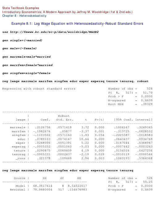
Stata Textbook ExamplesIntroductory Econometrics: A Modern Approach by Jeffrey M. Wooldridge (1st & 2nd eds.)Chapter 8 - HeteroskedasticityExample 8.1: Log Wage Equation with Heteroscedasticity-Robust Standard Errorsuse /ec-p/data/wooldridge/WAGE2gen single=(~married)gen male=(~female)gen marrmale=male*marriedgen marrfem=female*marriedgen singfem=single*femalereg lwage marrmale marrfem singfem educ exper expersq tenure tenursq, robustRegression with robust standard errors Number of obs = 526 F( 8, 517) = 51.70 Prob > F = 0.0000 R-squared = 0.4609 Root MSE = .39329------------------------------------------------------------------------------ | Robustlwage | Coef. Std. Err. t P>|t| [95% Conf. Interval] -------------+---------------------------------------------------------------- marrmale | .2126756 .0571419 3.72 0.000 .1004167 .3249345 marrfem | -.1982676 .05877 -3.37 0.001 -.313725 -.0828102 singfem | -.1103502 .0571163 -1.93 0.054 -.2225587 .0018583 educ | .0789103 .0074147 10.64 0.000 .0643437 .0934769 exper | .0268006 .0051391 5.22 0.000 .0167044 .0368967 expersq | -.0005352 .0001063 -5.03 0.000 -.0007442 -.0003263 tenure | .0290875 .0069409 4.19 0.000 .0154516 .0427234 tenursq | -.0005331 .0002437 -2.19 0.029 -.0010119 -.0000544 _cons | .321378 .109469 2.94 0.003 .1063193 .5364368 ------------------------------------------------------------------------------reg lwage marrmale marrfem singfem educ exper expersq tenure tenursqSource | SS df MS Number of obs = 526 -------------+------------------------------ F( 8, 517) = 55.25 Model | 68.3617614 8 8.54522017 Prob > F = 0.0000 Residual | 79.9680004 517 .154676983 R-squared = 0.4609Total | 148.329762 525 .28253288 Root MSE = .39329 ------------------------------------------------------------------------------ lwage | Coef. Std. Err. t P>|t| [95% Conf. Interval] -------------+---------------------------------------------------------------- marrmale | .2126756 .0553572 3.84 0.000 .103923 .3214283 marrfem | -.1982676 .0578355 -3.43 0.001 -.3118891 -.0846462 singfem | -.1103502 .0557421 -1.98 0.048 -.219859 -.0008414 educ | .0789103 .0066945 11.79 0.000 .0657585 .0920621 exper | .0268006 .0052428 5.11 0.000 .0165007 .0371005 expersq | -.0005352 .0001104 -4.85 0.000 -.0007522 -.0003183 tenure | .0290875 .006762 4.30 0.000 .0158031 .0423719 tenursq | -.0005331 .0002312 -2.31 0.022 -.0009874 -.0000789 _cons | .321378 .100009 3.21 0.001 .1249041 .517852 ------------------------------------------------------------------------------Example 8.2: Heteroscedastisity-Robust F Statisticsuse /ec-p/data/wooldridge/GPA3reg cumgpa sat hsperc tothrs female black white if term==2, robustRegression with robust standard errors Number of obs = 366 F( 6, 359) = 39.30 Prob > F = 0.0000 R-squared = 0.4006 Root MSE = .46929 ------------------------------------------------------------------------------ | Robustcumgpa | Coef. Std. Err. t P>|t| [95% Conf. Interval] -------------+---------------------------------------------------------------- sat | .0011407 .0001915 5.96 0.000 .0007641 .0015174 hsperc | -.0085664 .0014179 -6.04 0.000 -.0113548 -.0057779 tothrs | .002504 .0007406 3.38 0.001 .0010475 .0039605 female | .3034333 .0591378 5.13 0.000 .1871332 .4197334 black | -.1282837 .1192413 -1.08 0.283 -.3627829 .1062155 white | -.0587217 .111392 -0.53 0.598 -.2777846 .1603411 _cons | 1.470065 .2206802 6.66 0.000 1.036076 1.904053 ------------------------------------------------------------------------------reg cumgpa sat hsperc tothrs female black white if term==2Source | SS df MS Number of obs = 366Model | 52.831358 6 8.80522634 Prob > F = 0.0000 Residual | 79.062328 359 .220229326 R-squared = 0.4006 -------------+------------------------------ Adj R-squared = 0.3905 Total | 131.893686 365 .361352564 Root MSE = .46929 ------------------------------------------------------------------------------ cumgpa | Coef. Std. Err. t P>|t| [95% Conf. Interval] -------------+---------------------------------------------------------------- sat | .0011407 .0001786 6.39 0.000 .0007896 .0014919 hsperc | -.0085664 .0012404 -6.91 0.000 -.0110058 -.006127 tothrs | .002504 .000731 3.43 0.001 .0010664 .0039415 female | .3034333 .0590203 5.14 0.000 .1873643 .4195023 black | -.1282837 .1473701 -0.87 0.385 -.4181009 .1615335 white | -.0587217 .1409896 -0.42 0.677 -.3359909 .2185475 _cons | 1.470065 .2298031 6.40 0.000 1.018135 1.921994 ------------------------------------------------------------------------------Example 8.3: Heteroskedasticity-Robust LM Statisticuse /ec-p/data/wooldridge/CRIME1gen avgsensq=avgsen*avgsenreg narr86 pcnv avgsen avgsensq ptime86 qemp86 inc86 black hispan, robust Regression with robust standard errors Number of obs = 2725 F( 8, 2716) = 29.84 Prob > F = 0.0000 R-squared = 0.0728 Root MSE = .82843------------------------------------------------------------------------------ | Robustnarr86 | Coef. Std. Err. t P>|t| [95% Conf. Interval] -------------+---------------------------------------------------------------- pcnv | -.1355954 .0336218 -4.03 0.000 -.2015223 -.0696685 avgsen | .0178411 .0101233 1.76 0.078 -.0020091 .0376913 avgsensq | -.0005163 .0002077 -2.49 0.013 -.0009236 -.0001091 ptime86 | -.03936 .0062236 -6.32 0.000 -.0515634 -.0271566 qemp86 | -.0505072 .0142015 -3.56 0.000 -.078354 -.0226603 inc86 | -.0014797 .0002295 -6.45 0.000 -.0019297 -.0010296 black | .3246024 .0585135 5.55 0.000 .2098669 .439338 hispan | .19338 .0402983 4.80 0.000 .1143616 .2723985 _cons | .5670128 .0402756 14.08 0.000 .4880389 .6459867Source | SS df MS Number of obs = 2725 -------------+------------------------------ F( 2, 2723) = 2.00 Model | 3.99708536 2 1.99854268 Prob > F = 0.1355 Residual | 2721.00291 2723 .999266586 R-squared = 0.0015 -------------+------------------------------ Adj R-squared = 0.0007 Total | 2725.00 2725 1.00 Root MSE = .99963 ------------------------------------------------------------------------------ iota | Coef. Std. Err. t P>|t| [95% Conf. Interval] -------------+---------------------------------------------------------------- ur1 | .0277846 .0140598 1.98 0.048 .0002156 .0553537 ur2 | -.0010447 .0005479 -1.91 0.057 -.002119 .0000296 ------------------------------------------------------------------------------scalar hetlm = e(N)-e(rss)scalar pval = chi2tail(2,hetlm)display _n "Robust LM statistic : " %6.3f hetlm /*> */ _n "Under H0, distrib Chi2(2), p-value: " %5.3f pvalRobust LM statistic : 3.997Under H0, distrib Chi2(2), p-value: 0.136reg narr86 pcnv ptime86 qemp86 inc86 black hispanSource | SS df MS Number of obs = 2725 -------------+------------------------------ F( 6, 2718) = 34.95 Model | 143.977563 6 23.9962606 Prob > F = 0.0000 Residual | 1866.36959 2718 .686670196 R-squared = 0.0716 -------------+------------------------------ Adj R-squared = 0.0696 Total | 2010.34716 2724 .738012906 Root MSE = .82866 ------------------------------------------------------------------------------ narr86 | Coef. Std. Err. t P>|t| [95% Conf. Interval] -------------+---------------------------------------------------------------- pcnv | -.1322784 .0403406 -3.28 0.001 -.2113797 -.0531771 ptime86 | -.0377953 .008497 -4.45 0.000 -.0544566 -.021134 qemp86 | -.0509814 .0144359 -3.53 0.000 -.0792878 -.022675 inc86 | -.00149 .0003404 -4.38 0.000 -.0021575 -.0008224 black | .3296885 .0451778 7.30 0.000 .2411022 .4182748 hispan | .1954509 .0396929 4.92 0.000 .1176195 .2732823 _cons | .5703344 .0360073 15.84 0.000 .49973 .6409388 -----------------------------------------------------------------------------predict ubar2, residreg ubar2 pcnv avgsen avgsensq ptime86 qemp86 inc86 black hispanSource | SS df MS Number of obs = 2725 -------------+------------------------------ F( 8, 2716) = 0.43 Model | 2.37155739 8 .296444674 Prob > F = 0.9025 Residual | 1863.99804 2716 .686302664 R-squared = 0.0013 -------------+------------------------------ Adj R-squared = -0.0017 Total | 1866.36959 2724 .685157707 Root MSE = .82843 ------------------------------------------------------------------------------ ubar1 | Coef. Std. Err. t P>|t| [95% Conf. Interval] -------------+---------------------------------------------------------------- pcnv | -.003317 .0403699 -0.08 0.935 -.0824758 .0758418 avgsen | .0178411 .009696 1.84 0.066 -.0011713 .0368534 avgsensq | -.0005163 .000297 -1.74 0.082 -.0010987 .0000661 ptime86 | -.0015647 .0086935 -0.18 0.857 -.0186112 .0154819 qemp86 | .0004742 .0144345 0.03 0.974 -.0278295 .0287779 inc86 | .0000103 .0003405 0.03 0.976 -.0006574 .000678 black | -.0050861 .0454188 -0.11 0.911 -.094145 .0839729 hispan | -.0020709 .0397035 -0.05 0.958 -.0799229 .0757812 _cons | -.0033216 .0360573 -0.09 0.927 -.0740242 .0673809 ------------------------------------------------------------------------------scalar lm1 = e(N)*e(r2)display _n "LM statistic : " %6.3f lm1 /*LM statistic : 3.5425Example 8.4: Heteroscedasticity in Housing Price Equationuse /ec-p/data/wooldridge/HPRICE1reg price lotsize sqrft bdrmsSource | SS df MS Number of obs = 88 -------------+------------------------------ F( 3, 84) = 57.46 Model | 617130.701 3 205710.234 Prob > F = 0.0000 Residual | 300723.805 84 3580.0453 R-squared = 0.6724 -------------+------------------------------ Adj R-squared = 0.6607 Total | 917854.506 87 10550.0518 Root MSE = 59.833 ------------------------------------------------------------------------------ price | Coef. Std. Err. t P>|t| [95% Conf. Interval] -------------+----------------------------------------------------------------lotsize | .0020677 .0006421 3.22 0.002 .0007908 .0033446 sqrft | .1227782 .0132374 9.28 0.000 .0964541 .1491022 bdrms | 13.85252 9.010145 1.54 0.128 -4.06514 31.77018 _cons | -21.77031 29.47504 -0.74 0.462 -80.38466 36.84404 ------------------------------------------------------------------------------whitetst, fittedWhite's special test statistic : 16.26842 Chi-sq( 2) P-value = 2.9e-04reg lprice llotsize lsqrft bdrmsSource | SS df MS Number of obs = 88 -------------+------------------------------ F( 3, 84) = 50.42 Model | 5.15504028 3 1.71834676 Prob > F = 0.0000 Residual | 2.86256324 84 .034078134 R-squared = 0.6430 -------------+------------------------------ Adj R-squared = 0.6302 Total | 8.01760352 87 .092156362 Root MSE = .1846 ------------------------------------------------------------------------------ lprice | Coef. Std. Err. t P>|t| [95% Conf. Interval] -------------+---------------------------------------------------------------- llotsize | .1679667 .0382812 4.39 0.000 .0918404 .244093 lsqrft | .7002324 .0928652 7.54 0.000 .5155597 .8849051 bdrms | .0369584 .0275313 1.34 0.183 -.0177906 .0917074 _cons | -1.297042 .6512836 -1.99 0.050 -2.592191 -.0018931 ------------------------------------------------------------------------------whitetst, fittedWhite's special test statistic : 3.447243 Chi-sq( 2) P-value = .1784Example 8.5: Special Form of the White Test in the Log Housing Price Equationuse /ec-p/data/wooldridge/HPRICE1reg lprice llotsize lsqrft bdrmsSource | SS df MS Number of obs = 88 -------------+------------------------------ F( 3, 84) = 50.42 Model | 5.15506425 3 1.71835475 Prob > F = 0.0000 Residual | 2.86255771 84 .034078068 R-squared = 0.6430 -------------+------------------------------ Adj R-squared = 0.6302 Total | 8.01762195 87 .092156574 Root MSE = .1846llotsize | .167968 .0382811 4.39 0.000 .0918418 .2440941 lsqrft | .7002326 .0928652 7.54 0.000 .5155601 .8849051 bdrms | .0369585 .0275313 1.34 0.183 -.0177905 .0917075 _cons | 5.6107 .6512829 8.61 0.000 4.315553 6.905848 ------------------------------------------------------------------------------whitetst, fittedWhite's special test statistic : 3.447286 Chi-sq( 2) P-value = .1784Example 8.6: Family Saving Equationuse /ec-p/data/wooldridge/SAVINGreg sav incSource | SS df MS Number of obs = 100 -------------+------------------------------ F( 1, 98) = 6.49 Model | 66368437.0 1 66368437.0 Prob > F = 0.0124 Residual | 1.0019e+09 98 10223460.8 R-squared = 0.0621 -------------+------------------------------ Adj R-squared = 0.0526 Total | 1.0683e+09 99 10790581.8 Root MSE = 3197.4 ------------------------------------------------------------------------------ sav | Coef. Std. Err. t P>|t| [95% Conf. Interval] -------------+---------------------------------------------------------------- inc | .1466283 .0575488 2.55 0.012 .0324247 .260832 _cons | 124.8424 655.3931 0.19 0.849 -1175.764 1425.449 ------------------------------------------------------------------------------reg sav inc [aw = 1/inc](sum of wgt is 1.3877e-02)Source | SS df MS Number of obs = 100 -------------+------------------------------ F( 1, 98) = 9.14 Model | 58142339.8 1 58142339.8 Prob > F = 0.0032 Residual | 623432468 98 6361555.80 R-squared = 0.0853 -------------+------------------------------ Adj R-squared = 0.0760 Total | 681574808 99 6884594.02 Root MSE = 2522.2inc | .1717555 .0568128 3.02 0.003 .0590124 .2844986 _cons | -124.9528 480.8606 -0.26 0.796 -1079.205 829.2994 ------------------------------------------------------------------------------reg sav inc size educ age blackSource | SS df MS Number of obs = 100 -------------+------------------------------ F( 5, 94) = 1.70 Model | 88426246.4 5 17685249.3 Prob > F = 0.1430 Residual | 979841351 94 10423844.2 R-squared = 0.0828 -------------+------------------------------ Adj R-squared = 0.0340 Total | 1.0683e+09 99 10790581.8 Root MSE = 3228.6 ------------------------------------------------------------------------------ sav | Coef. Std. Err. t P>|t| [95% Conf. Interval] -------------+---------------------------------------------------------------- inc | .109455 .0714317 1.53 0.129 -.0323742 .2512842 size | 67.66119 222.9642 0.30 0.762 -375.0395 510.3619 educ | 151.8235 117.2487 1.29 0.199 -80.97646 384.6235 age | .2857217 50.03108 0.01 0.995 -99.05217 99.62361 black | 518.3934 1308.063 0.40 0.693 -2078.796 3115.583 _cons | -1605.416 2830.707 -0.57 0.572 -7225.851 4015.019 ------------------------------------------------------------------------------reg sav inc size educ age black [aw = 1/inc](sum of wgt is 1.3877e-02)Source | SS df MS Number of obs = 100 -------------+------------------------------ F( 5, 94) = 2.19 Model | 71020334.9 5 14204067.0 Prob > F = 0.0621 Residual | 610554473 94 6495260.35 R-squared = 0.1042 -------------+------------------------------ Adj R-squared = 0.0566 Total | 681574808 99 6884594.02 Root MSE = 2548.6 ------------------------------------------------------------------------------ sav | Coef. Std. Err. t P>|t| [95% Conf. Interval] -------------+---------------------------------------------------------------- inc | .1005179 .0772511 1.30 0.196 -.052866 .2539017 size | -6.868501 168.4327 -0.04 0.968 -341.2956 327.5586 educ | 139.4802 100.5362 1.39 0.169 -60.1368 339.0972 age | 21.74721 41.30598 0.53 0.600 -60.26678 103.7612 black | 137.2842 844.5941 0.16 0.871 -1539.677 1814.246 _cons | -1854.814 2351.797 -0.79 0.432 -6524.362 2814.734 ------------------------------------------------------------------------------Example 8.7: Demand for Cigarettesuse /ec-p/data/wooldridge/SMOKEreg cigs lincome lcigpric educ age agesq restaurnSource | SS df MS Number of obs = 807 -------------+------------------------------ F( 6, 800) = 7.42 Model | 8003.02506 6 1333.83751 Prob > F = 0.0000 Residual | 143750.658 800 179.688322 R-squared = 0.0527 -------------+------------------------------ Adj R-squared = 0.0456 Total | 151753.683 806 188.280003 Root MSE = 13.405 ------------------------------------------------------------------------------ cigs | Coef. Std. Err. t P>|t| [95% Conf. Interval] -------------+---------------------------------------------------------------- lincome | .8802689 .7277838 1.21 0.227 -.5483223 2.30886 lcigpric | -.7508498 5.773343 -0.13 0.897 -12.08354 10.58184 educ | -.5014982 .1670772 -3.00 0.003 -.8294597 -.1735368 age | .7706936 .1601223 4.81 0.000 .456384 1.085003 agesq | -.0090228 .001743 -5.18 0.000 -.0124443 -.0056013 restaurn | -2.825085 1.111794 -2.54 0.011 -5.007462 -.642708 _cons | -3.639884 24.07866 -0.15 0.880 -50.9047 43.62493 ------------------------------------------------------------------------------Change in cigs if income increases by 10%display _b[lincome]*10/100.08802689Turnover point for agedisplay _b[age]/2/_b[agesq]-42.708116whitetst, fittedWhite's special test statistic : 26.57258 Chi-sq( 2) P-value = 1.7e-06gen lubar=log(ub*ub)qui reg lubar lincome lcigpric educ age agesq restaurnpredict cigsh, xbgen cigse = exp(cigsh)reg cigs lincome lcigpric educ age agesq restaurn [aw=1/cigse](sum of wgt is 1.9977e+01)Source | SS df MS Number of obs = 807 -------------+------------------------------ F( 6, 800) = 17.06 Model | 10302.6415 6 1717.10692 Prob > F = 0.0000 Residual | 80542.0684 800 100.677586 R-squared = 0.1134 -------------+------------------------------ Adj R-squared = 0.1068 Total | 90844.71 806 112.710558 Root MSE = 10.034 ------------------------------------------------------------------------------ cigs | Coef. Std. Err. t P>|t| [95% Conf. Interval] -------------+---------------------------------------------------------------- lincome | 1.295241 .4370118 2.96 0.003 .4374154 2.153066 lcigpric | -2.94028 4.460142 -0.66 0.510 -11.69524 5.814684 educ | -.4634462 .1201586 -3.86 0.000 -.6993095 -.2275829 age | .4819474 .0968082 4.98 0.000 .2919194 .6719755 agesq | -.0056272 .0009395 -5.99 0.000 -.0074713 -.0037831 restaurn | -3.461066 .7955047 -4.35 0.000 -5.022589 -1.899543 _cons | 5.63533 17.80313 0.32 0.752 -29.31103 40.58169 ------------------------------------------------------------------------------Example 8.8: Labor Force Participation of Married Womenuse /ec-p/data/wooldridge/MROZreg inlf nwifeinc educ exper expersq age kidslt6 kidsge6Source | SS df MS Number of obs = 753 -------------+------------------------------ F( 7, 745) = 38.22 Model | 48.8080578 7 6.97257968 Prob > F = 0.0000 Residual | 135.919698 745 .182442547 R-squared = 0.2642 -------------+------------------------------ Adj R-squared = 0.2573 Total | 184.727756 752 .245648611 Root MSE = .42713 ------------------------------------------------------------------------------ inlf | Coef. Std. Err. t P>|t| [95% Conf. Interval] -------------+---------------------------------------------------------------- nwifeinc | -.0034052 .0014485 -2.35 0.019 -.0062488 -.0005616 educ | .0379953 .007376 5.15 0.000 .023515 .0524756exper | .0394924 .0056727 6.96 0.000 .0283561 .0506287 expersq | -.0005963 .0001848 -3.23 0.001 -.0009591 -.0002335 age | -.0160908 .0024847 -6.48 0.000 -.0209686 -.011213 kidslt6 | -.2618105 .0335058 -7.81 0.000 -.3275875 -.1960335 kidsge6 | .0130122 .013196 0.99 0.324 -.0128935 .0389179 _cons | .5855192 .154178 3.80 0.000 .2828442 .8881943 ------------------------------------------------------------------------------reg inlf nwifeinc educ exper expersq age kidslt6 kidsge6, robustRegression with robust standard errors Number of obs = 753 F( 7, 745) = 62.48 Prob > F = 0.0000 R-squared = 0.2642 Root MSE = .42713 ------------------------------------------------------------------------------ | Robustinlf | Coef. Std. Err. t P>|t| [95% Conf. Interval] -------------+---------------------------------------------------------------- nwifeinc | -.0034052 .0015249 -2.23 0.026 -.0063988 -.0004115 educ | .0379953 .007266 5.23 0.000 .023731 .0522596 exper | .0394924 .00581 6.80 0.000 .0280864 .0508983 expersq | -.0005963 .00019 -3.14 0.002 -.0009693 -.0002233 age | -.0160908 .002399 -6.71 0.000 -.0208004 -.0113812 kidslt6 | -.2618105 .0317832 -8.24 0.000 -.3242058 -.1994152 kidsge6 | .0130122 .0135329 0.96 0.337 -.013555 .0395795 _cons | .5855192 .1522599 3.85 0.000 .2866098 .8844287 ------------------------------------------------------------------------------Example 8.9: Determinants of Personal Computer Ownershipuse /ec-p/data/wooldridge/GPA1gen parcoll = (mothcoll | fathcoll)reg PC hsGPA ACT parcollSource | SS df MS Number of obs = 141 -------------+------------------------------ F( 3, 137) = 1.98 Model | 1.40186813 3 .467289377 Prob > F = 0.1201 Residual | 32.3569971 137 .236182461 R-squared = 0.0415 -------------+------------------------------ Adj R-squared = 0.0205 Total | 33.7588652 140 .241134752 Root MSE = .48599------------------------------------------------------------------------------ PC | Coef. Std. Err. t P>|t| [95% Conf. Interval] -------------+---------------------------------------------------------------- hsGPA | .0653943 .1372576 0.48 0.635 -.2060231 .3368118 ACT | .0005645 .0154967 0.04 0.971 -.0300792 .0312082 parcoll | .2210541 .092957 2.38 0.019 .037238 .4048702 _cons | -.0004322 .4905358 -0.00 0.999 -.970433 .9695686 ------------------------------------------------------------------------------predict phatgen h=phat*(1-phat)reg PC hsGPA ACT parcoll [aw=1/h](sum of wgt is 6.2818e+02)Source | SS df MS Number of obs = 141 -------------+------------------------------ F( 3, 137) = 2.22 Model | 1.54663033 3 .515543445 Prob > F = 0.0882 Residual | 31.7573194 137 .231805251 R-squared = 0.0464 -------------+------------------------------ Adj R-squared = 0.0256 Total | 33.3039497 140 .237885355 Root MSE = .48146 ------------------------------------------------------------------------------ PC | Coef. Std. Err. t P>|t| [95% Conf. Interval] -------------+---------------------------------------------------------------- hsGPA | .0327029 .1298817 0.25 0.802 -.2241292 .289535 ACT | .004272 .0154527 0.28 0.783 -.0262847 .0348286 parcoll | .2151862 .0862918 2.49 0.014 .04455 .3858224 _cons | .0262099 .4766498 0.05 0.956 -.9163323 .9687521 ------------------------------------------------------------------------------This page prepared by Oleksandr Talavera (revised 8 Nov 2002)Send your questions/comments/suggestions to Kit Baum at baum@ These pages are maintained by the Faculty Micro Resource Center's GSA Program,a unit of Boston College Academic Technology Services。
Chapter 8.ppt

Brand equity Building strong brands
Brand name selection Brand sponsorship Manufacturer’s brand Private brand Licensing Co-branding Brand development
Industrial products
Materials
products Shopping products Specialty products Unsought products
and parts Capital items Supplies and services
Group Assignment (Presentation 2)
制作一份品牌定位策划书; 设计某一品牌的名称和标志(品牌标识); 对某一产品进行包装设计; 为某一品牌设计新产品组合策略,实现品牌 延伸。
Describe the core, actual, and augmented levels of laptop.
Is Microsoft’s Windows XP professional operating software a product or a service? Describe the core, actual, and augmented levels of this software offering?
Organizations, Persons, Places, and Ideas
Product and Service Decisions
Individual product decisions Product line decisions Product mix decisions
动生电动势-感生电动势

• ••• ••••••
• • • • • • • • • •
• ••• ••••••
• • •
• • •
• • •
• •o •
•••
• R• •
••
• b•
••
• • •
• • •
R • • • • • • • • • •
• ••• ••••••
a • • • • • • • • • • B • • • • • • • • • •
i
dm
dt
B
dS
S t
i oa ab bo ab
ab
(b) Ei
(a)
dl
S
B
dS
t
a
其中 S 为 oabo 围成的面积。
P. 26 / 34 .
0
dl
Blv sin
若棒右移 ,则 i 指向:a
b;
a B
若棒左移,则 i 指向: b a。
Chapter 8. 电磁感应 §8. 2 动生作电者动:势杨感茂生田电动势
P. 9 / 34 .
例 如图,∞载流 I 直导线与导体棒相互垂直,棒以 v 沿
垂直于棒方向运动,已知:a、b。求导体棒的电动势。
(a) l
b v B
v
(vB sin 90o ) dl cos(90o )
0
dl a B
若 i > 0,则 i 指向与 dl 同向;否则,反向。
或
vB
在导体上的分量方向即为
i
指向。
Chapter 8. 电磁感应 §8. 2 动生作电者动:势杨感茂生田电动势
• ••• ••• •••
1 2
Chapter-8

⇒ c2 = 0
WL 3 W 4 WL3 ∴ EIy = x − x − x 12 24 24
Max occurs @ x = L /2 Max.
EIymax ∆ max
5WL4 =− 384 5WL4 = 384 EI
Example
y
x
P x
L P M= x 2 2 2 d y P L EI 2 = x f 0< x< for dx 2 2 dy P x 2 = + c1 EI Integrating g g d dx 2 2 L dy Since the beam is symmetric @ x= =0 2 dx 2 ⎛L⎞ ⎜ PL2 L P ⎝2⎠ c1 = − EI (0 ) = @ x= + c1 ⇒ 16 2 2 2 for 0 < x <
y x PL P L
Examples
x P
M = − PL + Px
d2y EI 2 = − PL + Px @ x dx x2 dy EI = − PLx + P + c1 Integrating once dx 2 2 ( dy 0) = 0 ⇒ EI (0 ) = − PL(0) + P + c1 ⇒ c1 = 0 @ x = 0 dx 2 2 3 PL PLx x Integrating twice EIy = − + P + c2 2 6 3 ( PL 2 0) @ x = 0 y = 0 ⇒ EI (0 ) = − (0) + P + c2 ⇒ c2 = 0 2 6
P 3 PL2 ∴ EIy = x − x 12 16
Max occurs @ x = L /2 Max.
Derivatives_Chapter 8

• Assume interest rates are unchanged
• The new swap price will be $22.483, $2 higher than the old one (check and understand why exactly $2)
• PV of the differences = 2/1.06 + 2/(1.0652) = $3.65
100,000 barrels are the notional amount of the swap, used to determine the magnitude of the payments when the swap is settled financially 10
Understanding Swaps
Strategy 1: Long forward contracts for 100,000 barrels in each of the next 2 years
• IP pays $20 in year one and $21 in year two for oil
Strategy 2: Prepaid swap
5
A Commodity Swap (cont’d)
Strategy 3: Swap
• Defer payments until the oil is delivered, while still fixing the total price • A swap usually calls for equal payment in each year
• Swap settlement; swap counterparty; market value of a swap; computing swap price (rate).
Chapter 8 对比分析和难度等级

02
03
04
Definition of Contrastive Analysis
Contrastive analysis is the systematic study of a pair of languages with a view to identifying their structural differences and similarities. Historically it has been used
Chapter 8 Contrastive Analysis, Interlanguage, and Error Analysis
Contrastive Analysis
01
The Contrastive Analysis Hypothesis (CAH) Hierarchy of Difficulty Moderating the Contrastive Analysis Hypothesis Markedness and Universal Grammer
How can we infer where the learner comes from?
Human learning theories
How do people interpret “interfering” elements of
learning with human learning theories?
to establish language genealogies. ---From Wikipedia
Definition of Contrastive Analysis
Contrastive analysis was used extensively in the field of second language acquisition in the 1960s and early 1970s, explaining why some features of a target language were more difficult to acquire than others. Therefore, the difficulty in mastering certain structures in a second language (L2) depended on the difference between the learners' mother language (L1) and the language they were trying to learn.
chapter8变电站馈线自动化

微机远动装置的基本功能
RTU的基本功能:遥测(YC)、遥信 (YX)、遥调(YT)、遥控(YK)。
RTU的辅助功能:屏幕显示、参数整定输 入、打印制表、信息转发功能、装置内 部功能、数据保存功能、事件顺序记录 功能。
1. “四遥”功能
1)遥信(YX):测量开关位置、保护动作信号、设备 运行状态信号,调压变压器分接头位置。一般用 无源接点,有变位时立即上传。
“开闭所”实际上就是相当于开关站,两进多出 (常用4~6出),只是根据不同的要求,进出 可以设置断路器、负荷开关或不设。没有断路 器或负荷开关的叫电缆分接箱,电缆直接进出, 用于小容量和用电可靠性不高的场所。“开闭 所”一般应采用断路器进(两进线设置BZT)、 负荷开关出。
远动装置(RTU)的发展
利用RTU微机功能,接入显示CRT或打印机,可就 地显示与参数输入整定,或一发多收。
RTU通信速率应可选择整定。 RTU应支持多种通信信道转接功能(如光端机、微
波、载波、无线电台等)。
微机远动装置的分类
RTU结构:集中式、分布式(功能分布式与结构分 布式)。
采样方式:直流、交流采样。 组屏方式:集中、分散组屏。
定义:与电源侧前级开关配合,失压或无电流时自 动分闸的开关设备。
功能:永久故障时,分合预定次数后闭锁在分闸状, 隔离故障区段;若未完成预定分合次数,故障已被 其他设备切除,则保持在合闸状(经一段延时后恢 复到预定状态,为下次故障作准备)。
要求:一般不能开断短路故障电流。 分类:电压—时间型,过流脉冲记数型。
SOE分辨率
事件分辨率要求达到毫秒级。 SOE站内分辨率:RTU内(站内)顺序发生一串事
件后,两事件间能辨认的最小时间,要求<5ms。 SOE站间分辨率:各RTU间(站间)顺序发生一串
Chapter08_其它常用工业控制器简介

ARM7
3 80 0.06 0.97 冯· 诺伊曼
ARM9
5 150 0.19 (+cache) 1.1 哈佛
ARM10
6 260 0.5 (+cache) 1.3 哈佛
ARM11
8 335 0.4 (+cache) 1.2 哈佛
机械电子工程学院
8.2 ARM的结构特点与工作原理
基于ARM内核的常用微处理器简介 ARM微处理器有多种内核结构,还有多种多样的内部 功能配置组合,在设计一个系统时选择最合适的ARM芯片 非常重要。 一些主流的ARM9处理器芯片如: – – – – – 飞思卡尔:MC9328MX27… 三星:S3C2440A … Atmel公司:AT91SAM9263 … 意法半导体:STR91x … 恩智浦半导体:LPC2000 系列…
备注 不能直接切换到其它模式
运行操作系统的特权 与用户模式类似,但具有可以直 任务 接切换到其它模式等特权
支持高速数据传输及 FIQ异常响应时进入此模式 通道处理
用于通用中断处理 IRQ异常响应时进入此模式 系统复位和软件中断响应时进入 此模式
管理 (svc)
中止 (abt) 未定义 (und)
操作系统保护模式
机械电子工程学院
8.1 DSP的结构特点与工作原理
• 系统复位后程序指针指向0000H处, 程序从该处开始执行,一般要在该处加一 条跳转指令使CPU自动转入用户程序的入 口。 • 0000H-003FH用于存储系统的中断 向量表,当有中断请求信号时,CPU从该 处取出中断子程序的入口地址。FLASH 的其他区域为用户程序区。 • 8000H-87FFH为单口存储器 (SARAM),仿真时,若程序较小,可将 程序代码放入该区。 • 8800H-FDFFH为用户扩展区。
Solutions - Chapter 8

Solutions - Chapter 88-1: MessageWrite a function called display_message() that prints one sentencetelling everyone what you are learning about in this chapter. Call the function, and make sure the message displays correctly.Output:8-2: Favorite BookWrite a function called favorite_book() that accepts oneparameter, title. The function should print a message, such as One of my favorite books is Alice in Wonderland. Call the function, making sure to include a book title as an argument in the function call.Output:8-3: T-ShirtWrite a function called make_shirt() that accepts a size and the textof a message that should be printed on the shirt. The function should print a sentence summarizing the size of the shirt and the message printed on it.Call the function once using positional arguments to make a shirt. Call the function a second time using keyword arguments.Output:8-4: Large ShirtsModify the make_shirt() function so that shirts are large by defaultwith a message that reads I love Python. Make a large shirt and a medium shirt with the default message, and a shirt of any size with a different message.Output:8-5: CitiesWrite a function called describe_city() that accepts the name of acity and its country. The function should print a simple sentence, suchas Reykjavik is in Iceland. Give the parameter for the country adefault value. Call your function for three different cities, at least one of which is not in the default country.Output:8-6: City NamesWrite a function called city_country() that takes in the name of a city and its country. The function should return a string formatted like this: “Santiago, Chile”Call your function with at least three city-country pairs, and print the value that’s returned.Output:8-7: AlbumWrite a function called make_album() that builds a dictionarydescribing a music album. The function should take in an artist name and an album title, and it should return a dictionary containing these two pieces of information. Use the function to make three dictionaries representing different albums. Print each return value to show that the dictionaries are storing the album information correctly.Add an optional parameter to make_album() that allows you to storethe nubmer of tracks on an album. If the calling line includes a value for the number of tracks, add that value to the album’s dictionary. Make at least one new function call that includes the nubmer of tracks on an album.Simple version:Output:With tracks:Output:8-8: User AlbumsStart with your program from Exercise 8-7. Write a while loop that allows users to enter an album’s artist and title. Once you have that information, call make_album()with the user’s input and print the dictionary that’s created. Be sure to include a quit value inthe while loop.Output:8-9: MagiciansMake a list of magician’s names. Pass the list to a functioncalled show_magicians(), wich prints the name of each magician in the list.Output:8-10: Great MagiciansStart with a copy of your program from Exercise 8-9. Write a function called make_great() that modifies the list of magicians by adding the phrase the Great to each magician’s name. Call show_magicians() to see that the list has actually been modified.Output:8-11: Unchanged MagiciansStart with your work from Exercise 8-10. Call thefunction make_great()with a copy of the list of magicians’ names.Because the original list will be unchanged, return the new list and store it in a separate list. Call show_magicians() with each list to showthat you have one list of the original names and one list with the Great added to each magician’s name.Output:8-12: SandwichesWrite a function that accepts a list of items a person wants on a sandwich. The function should have one parameter that collects as many items as the function call provides, and it should print a summary of the sandiwch that is being ordered. Call the function three tiems, using a different number of arguments each time.Output:8-14: CarsWrite a function that stores information about a car in a dictionary. the function should always receive a manufacturer and a model name. It should then accept an arbitrary number of keyword arguments. Call the function with the required information and two other name-value pairs, such as a color or an optional feature. Your function should work for a call like this one:car = make_car('subaru', 'outback', color='blue',tow_package=True)Print the dictionary that’s returned to make sure all the information was stored correctly.Output:8-15: Printing ModelsPut the functions for the example printing_models.py in a separate file called printing_functions.py. Write an import statement at the topof printing_models.py, and modify the file to use the imported functions.Note: The text refers to print_models.py, but it should sayprinting_models.py.printing_functions.py:printing_models.py:Output:。
国际财务管理课后习题答案chapter 8Word版

CHAPTER 8 MANAGEMENT OF TRANSACTION EXPOSURE SUGGESTED ANSWERS AND SOLUTIONS TO END-OF-CHAPTER QUESTIONS AND PROBLEMSQUESTIONS1. How would you define transaction exposure? How is it different from economic exposure?Answer: Transaction exposure is the sensitivity of realized domestic currency values of the firm’s contractual cash flows denominated in foreign currencies to unexpected changes in exchange rates. Unlike economic exposure, transaction exposure is well-defined and short-term.2. Discuss and compare hedging transaction exposure using the forward contract vs. money market instruments. When do the alternative hedging approaches produce the same result?Answer: Hedging transaction exposure by a forward contract is achieved by selling or buying foreign currency receivables or payables forward. On the other hand, money market hedge is achieved by borrowing or lending the present value of foreign currency receivables or payables, thereby creating offsetting foreign currency positions. If the interest rate parity is holding, the two hedging methods are equivalent.3. Discuss and compare the costs of hedging via the forward contract and the options contract.Answer: There is no up-front cost of hedging by forward contracts. In the case of options hedging, however, hedgers should pay the premiums for the contracts up-front. The cost of forward hedging, however, may be realized ex post when the hedger regrets his/her hedging decision.4. What are the advantages of a currency options contract as a hedging tool compared with the forward contract?Answer: The main advantage of using options contracts for hedging is that the hedger can decide whether to exercise options upon observing the realized future exchange rate. Options thus provide a hedge against ex post regret that forward hedger might have to suffer. Hedgers can only eliminate the downside risk while retaining the upside potential.5. Suppose your company has purchased a put option on the German mark to manage exchange exposure associated with an account receivable denominated in that currency. In this case, your company can be said to have an ‘insurance’ policy on its receivable. Explain in what sense this is so.Answer: Your company in this case knows in advance that it will receive a certain minimum dollar amount no matter what might happen to the $/€exchange rate. Furthermore, if the German mark appreciates, your company will benefit from the rising euro.6. Recent surveys of corporate exchange risk management practices indicate that many U.S. firms simply do not hedge. How would you explain this result?Answer: There can be many possible reasons for this. First, many firms may feel that they are not really exposed to exchange risk due to product diversification, diversified markets for their products, etc. Second, firms may be using self-insurance against exchange risk. Third, firms may feel that shareholders can diversify exchange risk themselves, rendering corporate risk management unnecessary.7. Should a firm hedge? Why or why not?Answer: In a perfect capital market, firms may not need to hedge exchange risk. But firms can add to their value by hedging if markets are imperfect. First, if management knows about the firm’s exposure better than shareholders, the firm, not its shareholders, should hedge. Second, firms may be able to hedge at a lower cost. Third, if default costs are significant, corporate hedging can be justifiable because it reduces the probability of default. Fourth, if the firm faces progressive taxes, it can reduce tax obligations by hedging which stabilizes corporate earnings.8. Using an example, discuss the possible effect of hedging on a firm’s tax obligations.Answer: One can use an example similar to the one presented in the chapter.9. Explain contingent exposure and discuss the advantages of using currency options to manage this type of currency exposure.Answer: Companies may encounter a situation where they may or may not face currency exposure. In this situation, companies need options, not obligations, to buy or sell a given amount of foreign exchange they may or may not receive or have to pay. If companies either hedge using forward contracts or do not hedge at all, they may face definite currency exposure.10. Explain cross-hedging and discuss the factors determining its effectiveness.Answer: Cross-hedging involves hedging a position in one asset by taking a position in another asset. The effectiveness of cross-hedging would depend on the strength and stability of the relationship between the two assets.PROBLEMS1. Cray Research sold a super computer to the Max Planck Institute in Germany on credit and invoiced €10 million payable in six months. Currently, the six-month forward exchange rate is $1.10/€ and the foreign exchange advisor for Cray Research predicts that the spot rate is likely to be $1.05/€ in six months.(a) What is the expected gain/loss from the forward hedging?(b) If you were the financial manager of Cray Research, would you recommend hedging this euro receivable? Why or why not?(c) Suppose the foreign exchange advisor predicts that the future spot rate will be the same as the forward exchange rate quoted today. Would you recommend hedging in this case? Why or why not?Solution: (a) Expected gain($) = 10,000,000(1.10 – 1.05)= 10,000,000(.05)= $500,000.(b) I would recommend hedging because Cray Research can increase the expected dollar receipt by $500,000 and also eliminate the exchange risk.(c) Since I eliminate risk without sacrificing dollar receipt, I still would recommend hedging.2. IBM purchased computer chips from NEC, a Japanese electronics concern, and was billed ¥250 million payable in three months. Currently, the spot exchange rate is ¥105/$ and the three-month forward rate is ¥100/$. The three-month money market interest rate is 8 percent per annum in the U.S. and 7 percent per annum in Japan. The management of IBM decided to use the money market hedge to deal with this yen account payable.(a) Explain the process of a money market hedge and compute the dollar cost of meeting the yen obligation.(b) Conduct the cash flow analysis of the money market hedge.Solution: (a). Let’s first compute the PV of ¥250 million, i.e.,250m/1.0175 = ¥245,700,245.7So if the above yen amount is invested today at the Japanese interest rate for three months, the maturity value will be exactly equal to ¥25 million which is the amount of payable.To buy the above yen amount today, it will cost:$2,340,002.34 = ¥250,000,000/105.The dollar cost of meeting this yen obligation is $2,340,002.34 as of today.(b)___________________________________________________________________Transaction CF0 CF1____________________________________________________________________1. Buy yens spot -$2,340,002.34with dollars ¥245,700,245.702. Invest in Japan - ¥245,700,245.70 ¥250,000,0003. Pay yens - ¥250,000,000Net cash flow - $2,340,002.34____________________________________________________________________3. You plan to visit Geneva, Switzerland in three months to attend an international business conference. You expect to incur the total cost of SF 5,000 for lodging, meals and transportation during your stay. As of today, the spot exchange rate is $0.60/SF and the three-month forward rate is $0.63/SF. You can buy the three-month call option on SF with the exercise rate of $0.64/SF for the premium of $0.05 per SF. Assume that your expected future spot exchange rate is the same as the forward rate. The three-month interest rate is 6 percent per annum in the United States and 4 percent per annum in Switzerland.(a) Calculate your expected dollar cost of buying SF5,000 if you choose to hedge via call option on SF.(b) Calculate the future dollar cost of meeting this SF obligation if you decide to hedge using a forward contract.(c) At what future spot exchange rate will you be indifferent between the forward and option market hedges?(d) Illustrate the future dollar costs of meeting the SF payable against the future spot exchange rate under both the options and forward market hedges.Solution: (a) Total option premium = (.05)(5000) = $250. In three months, $250 is worth $253.75 = $250(1.015). At the expected future spot rate of $0.63/SF, which is less than the exercise price, y ou don’t expect to exercise options. Rather, you expect to buy Swiss franc at $0.63/SF. Since you are going to buy SF5,000, you expect to spend $3,150 (=.63x5,000). Thus, the total expected cost of buying SF5,000 will be the sum of $3,150 and $253.75, i.e., $3,403.75.(b) $3,150 = (.63)(5,000).(c) $3,150 = 5,000x + 253.75, where x represents the break-even future spot rate. Solving for x, we obtain x = $0.57925/SF. Note that at the break-even future spot rate, options will not be exercised.(d) If the Swiss franc appreciates beyond $0.64/SF, which is the exercise price of call option, you will exercise the option and buy SF5,000 for $3,200. The total cost of buying SF5,000 will be $3,453.75 = $3,200 + $253.75.This is the maximum you will pay.4. Boeing just signed a contract to sell a Boeing 737 aircraft to Air France. Air France will be billed €20 million which is payable in one year. The current spot exchange rate is $1.05/€ and the one -year forward rate is $1.10/€. The annual interest rate is 6.0% in the U.S. and5.0% in France. Boeing is concerned with the volatile exchange rate between the dollar and the euro and would like to hedge exchange exposure.(a) It is considering two hedging alternatives: sell the euro proceeds from the sale forward or borrow euros from the Credit Lyonnaise against the euro receivable. Which alternative would you recommend? Why?(b) Other things being equal, at what forward exchange rate would Boeing be indifferent between the two hedging methods?Solution: (a) In the case of forward hedge, the future dollar proceeds will be (20,000,000)(1.10) = $22,000,000. In the case of money market hedge (MMH), the firm has to first borrow the PV of its euro receivable, i.e., 20,000,000/1.05 =€19,047,619. Then the firm should exchange this euro amount into dollars at the current spot rate to receive: (€19,047,619)($1.05/€) = $20,000,000, which can be invested at the dollar interest rate for one year to yield:$ Cost Options hedge Forward hedge $3,453.75 $3,150 0 0.579 0.64 (strike price) $/SF$253.75$20,000,000(1.06) = $21,200,000.Clearly, the firm can receive $800,000 more by using forward hedging.(b) According to IRP, F = S(1+i$)/(1+i F). Thus the “indifferent” forward rate will be:F = 1.05(1.06)/1.05 = $1.06/€.5. Suppose that Baltimore Machinery sold a drilling machine to a Swiss firm and gave the Swiss client a choice of paying either $10,000 or SF 15,000 in three months.(a) In the above example, Baltimore Machinery effectively gave the Swiss client a free option to buy up to $10,000 dollars using Swiss franc. What is the ‘implied’ exercise exchange rate?(b) If the spot exchange rate turns out to be $0.62/SF, which currency do you think the Swiss client will choose to use for payment? What is the value of this free option for the Swiss client?(c) What is the best way for Baltimore Machinery to deal with the exchange exposure?Solution: (a) The implied exercise (price) rate is: 10,000/15,000 = $0.6667/SF.(b) If the Swiss client chooses to pay $10,000, it will cost SF16,129 (=10,000/.62). Since the Swiss client has an option to pay SF15,000, it will choose to do so. The value of this option is obviously SF1,129 (=SF16,129-SF15,000).(c) Baltimore Machinery faces a contingent exposure in the sense that it may or may not receive SF15,000 in the future. The firm thus can hedge this exposure by buying a put option on SF15,000.6. Princess Cruise Company (PCC) purchased a ship from Mitsubishi Heavy Industry. PCC owes Mitsubishi Heavy Industry 500 million yen in one year. The current spot rate is 124 yen per dollar and the one-year forward rate is 110 yen per dollar. The annual interest rate is 5% in Japan and 8% in the U.S. PCC can also buy a one-year call option on yen at the strike price of $.0081 per yen for a premium of .014 cents per yen.(a) Compute the future dollar costs of meeting this obligation using the money market hedge and the forward hedges.(b) Assuming that the forward exchange rate is the best predictor of the future spot rate, compute the expected future dollar cost of meeting this obligation when the option hedge is used.(c) At what future spot rate do you think PCC may be indifferent between the option and forward hedge?Solution: (a) In the case of forward hedge, the dollar cost will be 500,000,000/110 = $4,545,455. In the case of money market hedge, the future dollar cost will be: 500,000,000(1.08)/(1.05)(124)= $4,147,465.(b) The option premium is: (.014/100)(500,000,000) = $70,000. Its future value will be $70,000(1.08) = $75,600.At the expected future spot rate of $.0091(=1/110), which is higher than the exercise of $.0081, PCC will exercise its call option and buy ¥500,000,000 for $4,050,000 (=500,000,000x.0081).The total expected cost will thus be $4,125,600, which is the sum of $75,600 and $4,050,000.(c) When the option hedge is used, PCC will spend “at most” $4,125,000. On the other hand, when the forward hedging is used, PCC will have to spend $4,545,455 regardless of the future spot rate. This means that the options hedge dominates the forward hedge. At no future spot rate, PCC will be indifferent between forward and options hedges.7. Airbus sold an aircraft, A400, to Delta Airlines, a U.S. company, and billed $30 million payable in six months. Airbus is concerned with the euro proceeds from international sales and would like to control exchange risk. The current spot exchange rate is $1.05/€ and six-month forward exchange rate is $1.10/€ at the moment. Airbus can buy a six-month put option on U.S. dollars with a strike price of€0.95/$ for a premium of €0.02 per U.S. dollar. Currently, six-month interest rate is 2.5% in the euro zone and 3.0% in theU.S.pute the guaranteed euro proceeds from the American sale if Airbus decides tohedge using a forward contract.b.If Airbus decides to hedge using money market instruments, what action doesAirbus need to take? What would be the guaranteed euro proceeds from the American sale in this case?c.If Airbus decides to hedge using put options on U.S. dollars, what would be the‘expected’ euro proceeds from the American sale? Assume that Airbus regards the current forward exchange rate as an unbiased predictor of the future spot exchange rate.d.At what future spot exchange rate do you think Airbus will be indifferent betweenthe option and money market hedge?Solution:a. Airbus will sell $30 million forward for €27,272,727 = ($30,000,000) / ($1.10/€).b. Airbus will borrow the present value of the dollar receivable, i.e., $29,126,214 = $30,000,000/1.03, and then sell the dollar proceeds spot for euros: €27,739,251. This is the euro amount that Airbus is going to keep.c. Since the expected future spot rate is less than the strike price of the put option, i.e., €0.9091< €0.95, Airbus expects to exercise the option and receive €28,500,000 = ($30,000,000)(€0.95/$). This is gross proceeds. Airbus spent €600,000 (=0.02x30,000,000) upfront for the option and its future cost is equal to €615,000 = €600,000 x 1.025. Thus the net euro proceeds from the American sale is €27,885,000, which is the difference between the gross proceeds and the option costs.d. At the indifferent future spot rate, the following will hold:€28,432,732 = S T(30,000,000) - €615,000.Solving for S T, we obtain the “indifference” future spot exchange rate, i.e., €0.9683/$, or $1.0327/€. Note that €28,432,732 is the future value of the proceeds under money market hedging:€28,432,732 = (€27,739,251) (1.025).Suggested solution for Mini Case: Chase Options, Inc.[See Chapter 13 for the case text]Chase Options, Inc.Hedging Foreign Currency Exposure Through Currency OptionsHarvey A. PoniachekI. Case SummaryThis case reviews the foreign exchange options market and hedging. It presents various international transactions that require currency options hedging strategies by the corporations involved. Seven transactions under a variety of circumstances are introduced that require hedging by currency options. The transactions involve hedging of dividend remittances, portfolio investment exposure, and strategic economic competitiveness. Market quotations are provided for options (and options hedging ratios), forwards, and interest rates for various maturities.II. Case Objective.The case introduces the student to the principles of currency options market and hedging strategies. The transactions are of various types that often confront companies that are involved in extensive international business or multinational corporations. The case induces students to acquire hands-on experience in addressing specific exposure and hedging concerns, including how to apply various market quotations, which hedging strategy is most suitable, and how to address exposure in foreign currency through cross hedging policies.III. Proposed Assignment Solution1. The company expects DM100 million in repatriated profits, and does not want the DM/$ exchange rate at which they convert those profits to rise above 1.70. They can hedge this exposure using DM put options with a strike price of 1.70. If the spot rate rises above 1.70, they can exercise the option, while if that rate falls they can enjoy additional profits from favorable exchange rate movements.To purchase the options would require an up-front premium of:DM 100,000,000 x 0.0164 = DM 1,640,000.With a strike price of 1.70 DM/$, this would assure the U.S. company of receiving at least:DM 100,000,000 – DM 1,640,000 x (1 + 0.085106 x 272/360)= DM 98,254,544/1.70 DM/$ = $57,796,791by exercising the option if the DM depreciated. Note that the proceeds from the repatriated profits are reduced by the premium paid, which is further adjusted by the interest foregone on this amount.However, if the DM were to appreciate relative to the dollar, the company would allow the option to expire, and enjoy greater dollar proceeds from this increase.Should forward contracts be used to hedge this exposure, the proceeds received would be:DM100,000,000/1.6725 DM/$ = $59,790,732,regardless of the movement of the DM/$ exchange rate. While this amount is almost $2 million more than that realized using option hedges above, there is no flexibilityregarding the exercise date; if this date differs from that at which the repatriate profits are available, the company may be exposed to additional further current exposure. Further, there is no opportunity to enjoy any appreciation in the DM.If the company were to buy DM puts as above, and sell an equivalent amount in calls with strike price 1.647, the premium paid would be exactly offset by the premium received. This would assure that the exchange rate realized would fall between 1.647 and 1.700. If the rate rises above 1.700, the company will exercise its put option, and if it fell below 1.647, the other party would use its call; for any rate in between, both options would expire worthless. The proceeds realized would then fall between:DM 100,00,000/1.647 DM/$ = $60,716,454andDM 100,000,000/1.700 DM/$ = $58,823,529.This would allow the company some upside potential, while guaranteeing proceeds at least $1 million greater than the minimum for simply buying a put as above.Buy/Sell OptionsDM/$Spot Put Payoff “Put”ProfitsCallPayoff“Call”Profits Net Profit1.60(1,742,846)01,742,84660,716,45460,716,4541.61(1,742,846)01,742,84660,716,45460,716,454 1.62(1,742,846)01,742,84660,716,45460,716,4541.63(1,742,846)01,742,84660,716,45460,716,4541.64(1,742,846)01,742,84660,716,4560,716,45441.65(1,742,846)60,606,061,742,846060,606,06111.66(1,742,846)60,240,961,742,846060,240,96441,742,846059,880,240 1.67(1,742,846)59,880,241.68(1,742,846)59,523,811,742,846059,523,8101,742,846059,171,598 1.69(1,742,846)59,171,5981.70(1,742,846)58,823,521,742,846058,823,52991,742,846058,823,529 1.71(1,742,846)58,823,5291.72(1,742,846)58,823,521,742,846058,823,52991,742,846058,823,529 1.73(1,742,846)58,823,5291.74(1,742,846)58,823,521,742,846058,823,52991,742,846058,823,529 1.75(1,742,846)58,823,5291.76(1,742,846)58,823,521,742,846058,823,52991.77(1,742,846)58,823,521,742,846058,823,52991.78(1,742,846)58,823,521,742,846058,823,52991.79(1,742,846)58,823,521,742,846058,823,52991,742,846058,823,5291.80(1,742,846)58,823,5291,742,846058,823,5291.81(1,742,846)58,823,5291.82(1,742,846)58,823,521,742,846058,823,52991,742,846058,823,5291.83(1,742,846)58,823,5291.84(1,742,846)58,823,521,742,846058,823,52991,742,846058,823,5291.85(1,742,846)58,823,529Since the firm believes that there is a good chance that the pound sterling will weaken, locking them into a forward contract would not be appropriate, because they would lose the opportunity to profit from this weakening. Their hedge strategy should follow for an upside potential to match their viewpoint. Therefore, they should purchase sterling call options, paying a premium of:5,000,000 STG x 0.0176 = 88,000 STG.If the dollar strengthens against the pound, the firm allows the option to expire, and buys sterling in the spot market at a cheaper price than they would have paid for a forward contract; otherwise, the sterling calls protect against unfavorable depreciation of the dollar.Because the fund manager is uncertain when he will sell the bonds, he requires a hedge which will allow flexibility as to the exercise date. Thus, options are the best instrument for him to use. He can buy A$ puts to lock in a floor of 0.72 A$/$. Since he is willing to forego any further currency appreciation, he can sell A$ calls with a strike price of 0.8025 A$/$ to defray the cost of his hedge (in fact he earns a net premium of A$ 100,000,000 x (0.007234 – 0.007211) = A$ 2,300), while knowing that he can’t receive less than 0.72 A$/$ when redeeming his investment, and can benefit from a small appreciation of the A$.Example #3:Problem: Hedge principal denominated in A$ into US$. Forgo upside potential to buy floor protection.I. Hedge by writing calls and buying puts1) Write calls for $/A$ @ 0.8025Buy puts for $/A$ @ 0.72# contracts needed = Principal in A$/Contract size100,000,000A$/100,000 A$ = 1002) Revenue from sale of calls = (# contracts)(size of contract)(premium)$75,573 = (100)(100,000 A$)(.007234 $/A$)(1 + .0825 195/360)3) Total cost of puts = (# contracts)(size of contract)(premium)$75,332 = (100)(100,000 A$)(.007211 $/A$)(1 + .0825 195/360)4) Put payoffIf spot falls below 0.72, fund manager will exercise putIf spot rises above 0.72, fund manager will let put expire5) Call payoffIf spot rises above .8025, call will be exercised If spot falls below .8025, call will expire6) Net payoffSee following Table for net payoffAustralian Dollar Bond HedgeStrikePrice Put Payoff “Put”PrincipalCallPayoff“Call”Principal Net Profit0.60(75,332)72,000,0075,573072,000,2410.61(75,332)72,000,0075,573072,000,2410.62(75,332)72,000,0075,573072,000,2410.63(75,332)72,000,0075,573072,000,2410.64(75,332)72,000,0075,573072,000,2410.65(75,332)72,000,0075,573072,000,2410.66(75,332)72,000,0075,573072,000,2410.67(75,332)72,000,0075,573072,000,2410.68(75,332)72,000,0075,573072,000,2410.69(75,332)72,000,0075,573072,000,2410.70(75,332)72,000,0075,573072,000,2410.71(75,332)72,000,0075,573072,000,2410.72(75,332)72,000,0075,573072,000,2410.73(75,332)73,000,0075,573073,000,2410.74(75,332)74,000,0075,573074,000,2410.75(75,332)75,000,0075,573075,000,2410.76(75,332)76,000,0075,573076,000,24175,573077,000,2410.77(75,332)77,000,000.78(75,332)78,000,0075,573078,000,24175,573079,000,2410.79(75,332)79,000,000.80(75,332)80,000,0075,573080,000,24180,250,2410.81(75,332)075,57380,250,000.82(75,332)075,57380,250,0080,250,24180,250,2410.83(75,332)075,57380,250,000.84(75,332)075,57380,250,0080,250,24180,250,2410.85(75,332)075,57380,250,004. The German company is bidding on a contract which they cannot be certain of winning. Thus, the need to execute a currency transaction is similarly uncertain, and using a forward or futures as a hedge is inappropriate, because it would force them to perform even if they do not win the contract.Using a sterling put option as a hedge for this transaction makes the most sense. Fora premium of:12 million STG x 0.0161 = 193,200 STG,they can assure themselves that adverse movements in the pound sterling exchange rate will not diminish the profitability of the project (and hence the feasibility oftheir bid), while at the same time allowing the potential for gains from sterling appreciation.5. Since AMC in concerned about the adverse effects that a strengthening of the dollar would have on its business, we need to create a situation in which it will profit from such an appreciation. Purchasing a yen put or a dollar call will achieve this objective. The data in Exhibit 1, row 7 represent a 10 percent appreciation of the dollar (128.15 strike vs. 116.5 forward rate) and can be used to hedge against a similar appreciation of the dollar.For every million yen of hedging, the cost would be:Yen 100,000,000 x 0.000127 = 127 Yen.To determine the breakeven point, we need to compute the value of this option if the dollar appreciated 10 percent (spot rose to 128.15), and subtract from it the premium we paid. This profit would be compared with the profit earned on five to 10 percent of AMC’s sales (which would be lost as a result of the dollar appreciation). The number of options to be purchased which would equalize these two quantities would represent the breakeven point.Example #5:Hedge the economic cost of the depreciating Yen to AMC.If we assume that AMC sales fall in direct proportion to depreciation in the yen (i.e., a 10 percent decline in yen and 10 percent decline in sales), then we can hedge the full value of AMC’s sales. I have a ssumed $100 million in sales.1) Buy yen puts# contracts needed = Expected Sales *Current ¥/$ Rate / Contract size9600 = ($100,000,000)(120¥/$) / ¥1,250,0002) Total Cost = (# contracts)(contract size)(premium)$1,524,000 = (9600)( ¥1,250,000)($0.0001275/¥)3) Floor rate = Exercise – Premium128.1499¥/$ = 128.15¥/$ - $1,524,000/12,000,000,000¥4) The payoff changes depending on the level of the ¥/$ rate. The following tablesummarizes the payoffs. An equilibrium is reached when the spot rate equals the floor rate.AMC ProfitabilityYen/$ Spot Put Payoff Sales Net Profit 120(1,524,990)100,000,00098,475,010 121(1,524,990)99,173,66497,648,564 122(1,524,990)98,360,65696,835,666 123(1,524,990)97,560,97686,035,986 124(1,524,990)96,774,19495,249,204 125(1,524,990)96,000,00094,475,010 126(1,524,990)95,238,09593,713,105 127(847,829)94,488,18993,640,360 128(109,640)93,750,00093,640,360 129617,10493,023,25693,640,360 1301,332,66892,307,69293,640,360 1312,037,30791,603,05393,640,360 1322,731,26990,909,09193,640,360 1333,414,79690,225,66493,640,360 1344,088,12289,552,23993,640,360 1354,751,43188,888,88993,640,360 1365,405,06688,235,29493,640,360 1376,049,11887,591,24193,640,360 1386,683,83986,966,52293,640,360 1397,308,42586,330,93693,640,360 1407,926,07585,714,28693,640,360 1418,533,97785,106,38393,640,360 1429,133,31884,507,04293,640,360 1439,724,27683,916,08493,640,360 14410,307,02783,333,33393,640,360 14510,881,74082,758,62193,640,360 14611,448,57982,191,78193,640,360。
交流传动控制系统

交流传动控制系统的历史与发展
早期的交流传动控制系统主要采用模拟电路和控制技术,随 着计算机技术和数字信号处理技术的不断发展,现代的交流 传动控制系统已经逐步实现数字化和智能化。
目前,交流传动控制系统正朝着高效率、高精度、高可靠性 和网络化方向发展,未来还将进一步融合人工智能、物联网 和云计算等先进技术,实现更加智能化和自动化的控制。
其他领域
总结词
除了上述领域外,交流传动控制系统还广泛 应用于电梯、压缩机、泵等机械设备中,提 高设备的运行效率和节能效果。
详细描述
在电梯中,交流传动控制系统用于控制电梯 的运行速度和平衡状态,提高电梯的安全性 和舒适度。在压缩机和泵等机械设备中,交 流传动控制系统可以实现精确的速度和压力
控制,提高设备的运行效率和节能效果。
02 交流传动控制系统的基本原理
CHAPTER
交流电机的工作原理
交流电机的基本结构
交流电机的调速原理
交流电机主要由定子和转子组成,通 过磁场相互作用实现能量的转换。
通过改变交流电的频率或相位,可以 改变旋转磁场的转速,从而实现对交 流电机的调速。
交流电机的旋转原理
当交流电通过定子绕组时,产生旋转 磁场,该磁场与转子相互作用,使转 子旋转。
维护保养
交流传动控制系统的维护保养相对复杂,需要专业技术人员进行 故障排查和维修。
对未来的展望
技术发展
随着电力电子技术和控制理论的不断进步,交流传动控制系统的性 能将得到进一步提升,实现更加精确、快速和智能的控制。
应用领域拓展
随着环保和节能要求的提高,交流传动控制系统将在更多领域得到 应用,如电动汽车、可再生能源等领域。
- 1、下载文档前请自行甄别文档内容的完整性,平台不提供额外的编辑、内容补充、找答案等附加服务。
- 2、"仅部分预览"的文档,不可在线预览部分如存在完整性等问题,可反馈申请退款(可完整预览的文档不适用该条件!)。
- 3、如文档侵犯您的权益,请联系客服反馈,我们会尽快为您处理(人工客服工作时间:9:00-18:30)。
sE 20 2 2 R2 ( sX 20 )
R2
2 R2 ( sX 20 ) 2
由前面分析知: cos 2
U1 4.44 f1 N1Φm
由此得电磁转矩公式
sR2 2 TK 2 U1 2 R2 ( sX 20 )
总目录 章目录 返回 上一页 下一页
电磁转矩公式
sR2 2 TK 2 U1 2 R2 ( sX 20 )
电动机的分类: 同步电动机 交流电动机 电动机 直流电动机 异步电动机 三相电动机 单相电动机
他励、并励电动机
串励、复励电动机
鼠笼式异步交流电动机授课内容: 基本结构、工作原理、 机械特性、控制方法
总目录 章目录 返回 上一页 下一页
8.1 三相异步电动机的构造
1.定子
铁心:由内周有槽 的硅钢片叠成。
同步转速 每个电流周期 磁场转过的空间角度 ( f1 50Hz )
p 1
p2
p3
p4
360
180
3000(转/分)
1500(转/分)
120
1000(转/分)
750 (转/分 )
总目录 章目录 返回 上一页 下一页
90
可见: 旋转磁场转速n0与频率f1和极对数p有关。
8. 2. 2 电动机的转动原理
由公式可知
2 1. T 与定子每相绕组电压 U 1 成正比。U 1 T
2. 当电源电压 U1 一定时,T 是 s 的函数。 3. R2 的大小对 T 有影响。绕线式异步电动机可外 接电阻来改变转子电阻R2 ,从而改变转距。
总目录 章目录 返回
上一页 下一页
8. 4. 2 机械特性曲线
根据转矩公式 得特性曲线: 动画 T
n0 60 f1 (转/分) 0 o 工频: f1 50 Hz
Im I m
i i A
i B iC
S
t
n0 3000 (转/分)
A Y C
N
Z Y B
A
A
S
C N
Z
Y B C
N
Z B
S
S
X
X
X
上一页 下一页
总目录 章目录 返回
p=2时
C
X
Y
A
N
30
Z
C
B
Y
A
Z
B
S
Z
转子电路的功率因数 I2, cos 2 I2
R ( sX 20 ) (n s cos 2 )
2 2 2
cos 2
R2
cos2
O
1
s
结论:转子转动时,转 子电路中的各量均与转 差率 s有关,即与转速 n有关。
总目录 章目录 返回 上一页 下一页
8.4 三相异步电动机转矩与机械特性
动画
t
iB B
iC
Y X Z C
Z
A A
A A
S
Y
Z C
Y
S
结论: 任意调换两根 电源进线,则旋转 磁场反转。
N
B
C
B
N
X
X
t 0
总目录 章目录 返回
t 60
上一页 下一页
3.旋转磁场的极对数P
iA
A
Z X Y
Im
i i A
i B iC
t
A Z
o
B
Y
iC C
iB
N
当三相定子绕组按 图示排列时,产生一对 磁极的旋转磁场,即:
S
A
X
S
N
S
B
n0
X
N
B
X
Y
C
Z
N
A Y
C
Im
i i A i B iC
t 0
t 60
0
t
60 f1 n0 1500 (转/分) 2
总目录 章目录 返回 上一页 下一页
旋转磁场转速n0与极对数 p 的关系 60 f1 n0 (转/分) p 极对数
8.2 三相异步电动机的转动原理
总目录 章目录 返回
上一页 下一页
8. 2. 1 旋转磁场
1.旋转磁场的产生 定子三相绕组通入三 相交流电(星形联接)
iA
i A I m sint iB I m sint 120 iC I m sint 120
Im
A Z X Y
三相绕组
A ----X B ----Y C---- Z
机座:铸钢或铸铁
总目录 章目录 返回
上一页 下一页
2.转子
鼠笼式
绕线式 鼠笼转子
铁心:由外周有槽的硅钢片叠成。 (1) 鼠笼式转子
铁芯槽内放铜条,端 部用短路环形成一体。 或铸铝形成转子绕组。 (2) 绕线式转子 同定子绕组一样,也分为三相,并且接成星形。 转子: 在旋转磁场作用下,产生感应电动势或电 流。
8. 4. 1 转矩公式
转子中各载流导体在旋转磁场的作用下,受到 电磁力所形成的转矩之总和。
F Bl i
T Φ , I 2 , cos 2
T K TΦI 2 cos 2
常数,与电 机结构有关 旋转磁场 每极磁通 转子电流 转子电路的 功率因数
总目录 章目录 返回ห้องสมุดไป่ตู้上一页 下一页
T KT Φ I 2 cos 2
总目录 章目录 返回 上一页 下一页
总目录 章目录 返回
上一页 下一页
鼠笼式电动机与绕线式电动机的的比较: 鼠笼式: 结构简单、价格低廉、工作可靠;不能人为改 变电动机的机械特性。
绕线式: 结构复杂、价格较贵、维护工作量大;转子 外加电阻可人为改变电动机的机械特性。
总目录 章目录 返回
上一页 下一页
n0 n n0 n n0 p f2 p s f1 60 n0 60
总目录 章目录 返回 上一页 下一页
2. 转子感应电动势E 2
E2= 4.44 f 2N2 = 4.44s f 1N2
即E2= s E20
转子转动时 的感应电势
当转速 n = 0(s=1)时, f 2最高,且 E2 最大,有
Φ U1
2.定子感应电势的频率 f1 感应电势的频率与磁场和导体间的相对速度有关 旋转磁场与定子导体间的相对速度为 n0 ,所以
pn0 f1 60
f 1= 电源频率 f
总目录 章目录 返回 上一页 下一页
8. 3. 2 转子电路
1. 转子感应电势频率 f 2 ∵定子导体与旋转磁场间的相对速度固定,而转子 导体与旋转磁场间的相对速度随转子的转速不同而 变化 旋转磁场切割定子导体和转子导体的速度不同 定子感应电势频率 f 1 转子感应电势频率 f 2 转子感应电势频率 f 2
n0 n s 100% 1000 975 100% 2.5% 1000 n0
总目录 章目录 返回
上一页 下一页
8.3 三相异步电动机的电路分析
三相异步电动机的电 磁关系与变压器类似。 变压器: 变化 e U1 E1= 4.44 f N1 E2= 4.44 f N2 E1 、E2 频率相同,都等 于电源频率。
I2
E2 R X sE 20
2 2 2 2
s 0 I 2 0 (n n0 )
R X 5. 转子电路的功率因数 cos2 s很小时 R2 SX 20 R2
2 2
2 R2 ( sX 20 ) 2
s 1 I 2max
E 20
2 20
cos 2
2 2 R2 X2 R2 2
总目录 章目录 返回 上一页 下一页
n (1 s )n0 异步电动机运行中: s (1 ~ 9)%
n0 n s 转差率s n 100% 0 转子转速亦可由转差率求得
例1:一台三相异步电动机,其额定转速 n=975 r/min,电源频率 f1=50 Hz。试求电动机的 极对数和额定负载下的转差率。 解: 根据异步电动机转子转速与旋转磁场同步转 速的关系可知:n0=1000 r/min , 即 p=3 额定转差率为
n
P P T 9550 2 πn n 额定转矩 60
PN (千瓦) TN 9550 nN (转 / 分)
O
TN
T
(N • m)
如某普通机床的主轴电机(Y132M-4型) 的额定功 率为7.5kw, 额定转速为1440r/min, 则额定转矩为 PN 7.5 TN 9550 9550 49.7 N . m nN 1440
cos 2 1
s较大时 R2 sX 20
cos 2
总目录 章目录 返回
R ( sX 20 )
2 2
1
s
上一页 下一页
转子绕组的感应电流
I 2、cos 2 随S变化曲线
E2
sE20 I2 2 2 2 2 ( n s I 2 ) R2 X 2 R2 ( sX 20 )
i1
i2
+
u1
-
e1
+ -
-
-
e2
+
-
+
e 1
+ f1
e 2
f2
U1 4.44 f N 1
异步电动机每相电路
总目录 章目录 返回
上一页 下一页
8. 3. 1 定子电路
1.旋转磁场的磁通 异步电动机:旋转磁场切割导体 e, U1 E1= 4.44 f 1N1 每极磁通 U
1