时间序列分析第四次作业房青B新编
时间序列分析第四次作业 ——房青 B0712094 1071209153
1. ARMA-GARCH modeling of SSE Composite Index. Use the recent 1000 obervations on the log return of the SSECI.
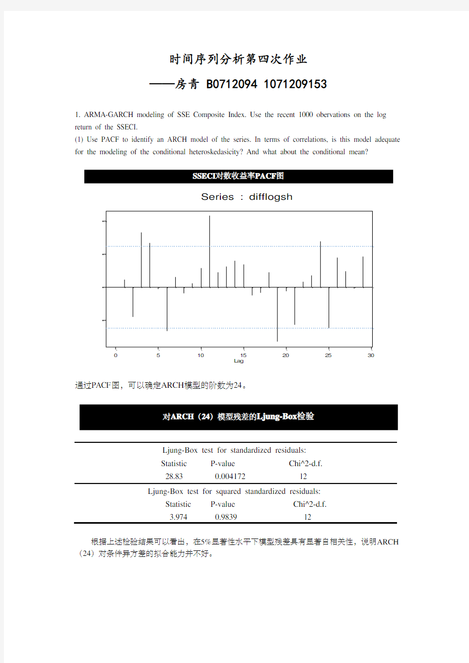
(1) Use PACF to identify an ARCH model of the series. In terms of correlations, is this model adequate for the modeling of the conditional heteroskedasicity? And what about the conditional mean?
Lag
P a r t i a l A C F 0
510
15202530
-0.05
0.0
0.05
0.1
0 Series : difflogsh
通过PACF 图,可以确定ARCH 模型的阶数为24。
Ljung-Box test for standardized residuals:
Statistic P-value Chi^2-d.f. 28.83 0.004172 12
Ljung-Box test for squared standardized residuals:
Statistic P-value Chi^2-d.f. 3.974 0.9839 12
根据上述检验结果可以看出,在5%显著性水平下模型残差具有显著自相关性,说明ARCH (24)对条件异方差的拟合能力并不好。
-4-2
2
4
-2
2
Quantiles of gaussian distribution
S t a n d a r d i z e d R e s i d u a l s
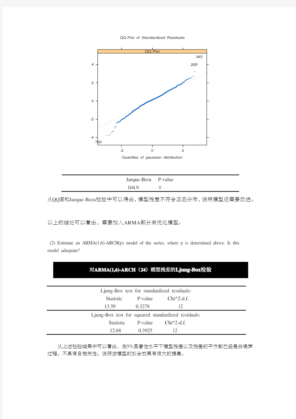
QQ-Plot of Standardized Residuals
Jarque-Bera P-value 104.9 0
从QQ 图和Jarque-Bera 检验中可以得出,模型残差不符合正态分布,说明模型还需要改进。
以上的结论可以看出,需要加入ARMA 部分来优化模型。
(2) Estimate an ARMA(1,6)-ARCH(p) model of the series, where p is determined above. Is this model adequate?
Ljung-Box test for standardized residuals:
Statistic P-value Chi^2-d.f. 13.59 0.3278 12 Ljung-Box test for squared standardized residuals:
Statistic P-value Chi^2-d.f. 12.68 0.3925 12
从上述检验结果中可以看出,在5%显著性水平下模型残差以及残差的平方都已经是白噪声过程,不具有自相关性。说明该模型的拟合效果有很大的提高。
-5
5
-2
2
Quantiles of gaussian distribution
S t a n d a r d i z e d R e s i d u a l s
QQ-Plot of Standardized Residuals
Jarque-Bera P-value 2205 0
虽然仍没有通过Jarque-Bera 检验,但是从QQ 图上来看,残差对正态分布的趋近程度
比上个模型大大提高了。
说明加入了ARMA 部分后,模型的拟合能力提高很大。
(3) Estimate a GARCH(1,1) model of the series. Is this model adequate for the conditional heteroskedasicity? What about the conditional mean?
Ljung-Box test for standardized residuals: Statistic P-value Chi^2-d.f. 30.93 0.002018 12 Ljung-Box test for squared standardized residuals:
Statistic P-value Chi^2-d.f. 10.4 0.5807 12
根据上述检验结果可以看出,在5%显著性水平下模型残差具有显著的自相关性,说明该
模型对条件异方差的拟合能力并不好。
Jarque-Bera P-value
146.2 0
-4-2
2
4
-2
2
Quantiles of gaussian distribution
S t a n d a r d i z e d R e s i d u a l s
QQ-Plot of Standardized Residuals
从QQ 图和Jarque-Bera 检验中可以得出,模型残差不符合正态分布,说明模型还需要改进。
以上的结论可以看出,需要加入ARMA 部分来优化模型。
(4) Estimate an ARMA(1,6)-GARCH(1,1) model of the series. Plot(i) Conditional Standard Deviations, sigma_t (ii) ACF of Standardized Residuals, \hat\varepsilon_t (iii) QQ-Plot of Standardized Residuals.
Ljung-Box test for standardized residuals:
Statistic P-value Chi^2-d.f.
13.73 0.3181 12 Ljung-Box test for squared standardized residuals:
Statistic P-value Chi^2-d.f. 9.298 0.6773 12
从上述检验结果中可以看出,在5%显著性水平下模型残差以及残差的平方都已经是白噪声
过程,不具有自相关性。说明该模型的拟合效果有很大的提高。
(i) Conditional Standard Deviations
0.010
0.015
0.020
0.025
0.030
0.035
200
400
600
800
1000
C o n d i t i o n a l S D
GARCH Volatility
从sigma_t 的图中可以推出,σt^2 即条件异方差正变得越来越大。随着股市从06年开始逐渐进入牛市格局,市场的波动率也逐渐变大。疯涨,暴跌,也是最近股市经常出现的事情,这样也就不难理解该图了。 (ii)
0.0
0.2
0.4
0.6
0.8
1.0
0510********
Lags
ACF of Std. Residuals
从ACF 图中可以看出残差的自相关性已经不明显了。
(iii) QQ-Plot of Standardized Residuals
-4-2
2
4
6
-2
2
Quantiles of gaussian distribution
S t a n d a r d i z e d R e s i d u a l s
QQ-Plot of Standardized Residuals
从QQ 图中发现残差并不服从正态分布。
(5) Estimate an ARMA(1,6)-GARCH(1,1) model with Student-t distribution. Plot QQ-Plot of
Standardized Residuals.
Ljung-Box test for standardized residuals:
Statistic P-value Chi^2-d.f. 11.94 0.4504 12 Ljung-Box test for squared standardized residuals:
Statistic P-value Chi^2-d.f. 8.658 0.7318 12
从上述检验结果中可以看出,在5%显著性水平下模型残差以及残差的平方都已经是白噪声过程,不具有自相关性。
-4-2
2
4
6
-6-4-20246
Quantiles of t distribution
S t a n d a r d i z e d R e s id u a l s
QQ-Plot of Standardized Residuals
从QQ 图中可以看出,残差基本服从T 学生分布。
2. Extensions of GARCH models. First use the above SSECI data.
(1) Estimate an ARMA(1,6)-GARCH-M(1,1) model of the SSECI series. Is the GARCH-M effect
significant?
Value Std.Error t value Pr(>|t|)
ARCH-IN-MEAN 4.414e+000 4.839e+000 0.9121 3.619e-001
可以看出,该模型的风险溢价参数在5%显著性水平下并不显著为正,说明上证市场投资者对风险补偿的要求并不明显。
对此结论可能的解释有,国内市场的最大特点即为投机气氛较浓厚,与国外市场大部分投资者注重稳定的价值性投资有所不同。市场上ST股票只要稍稍有些题材和故事,就很容易成为被市场所热炒的对象,但是这类上市公司经重组,注资后表现如何,还是要大打问号的。而且市场上很多散户并不理性,对于股市知之甚少,一味追涨杀跌,对于股市的风险性并没有较清醒的认识。
以上对模型结果的一些解释仅为个人观点。
Ljung-Box test for standardized residuals:
Statistic P-value Chi^2-d.f.
13.83 0.3114 12
Ljung-Box test for squared standardized residuals:
Statistic P-value Chi^2-d.f.
9.143 0.6906 12
从上述检验结果中可以看出,在5%显著性水平下模型残差以及残差的平方都已经是白噪声过程,不具有自相关性。
Value Std.Error t value Pr(>|t|)
LEV(1) -0.06913960 0.06959055 -0.9935 3.207e-001
在5%显著性水平下模型的LEV(1)并不显著,并没有得出负冲击对市场冲击更大的结论。
诚然,从去年530印花税导致的市场暴跌,到最近由于市场对我国经济增长和上市公司利润增长的怀疑以及市场扩容压力所导致的市场大面积暴跌,都说明负冲击对市场影响的强大威力性。
但是,市场同样容易对正面利好消息产生强烈反应,诸如最近印花税下调,股市一片红,消息公布次日涨停无数,股评师纷纷看到至少3800以上,市场公司盈利情况并未发生根本性改变,市场却做出如此巨大的反应,也足见正面利好对目前股市的冲击能力之大。
除此之外,市场上很有些人喜欢炒作行业题材,讲究板块理念,一条行业政策消息就能有效带动整个行业板块的上涨,也可以看出正面消息对市场的影响之大。
Ljung-Box test for standardized residuals:
Statistic P-value Chi^2-d.f.
13.2 0.3548 12
Ljung-Box test for squared standardized residuals:
Statistic P-value Chi^2-d.f.
8.808 0.7192 12
从上述检验结果中可以看出,在5%显著性水平下模型残差以及残差的平方都已经是白噪声过程,不具有自相关性。
Value Std.Error t value Pr(>|t|)
LEV(1) -0.103748 0.078326 -1.32456 1.856e-001
同样,在5%显著性水平下模型的LEV(1)并不显著,并没有得出负冲击对市场冲击更大的结论。
Ljung-Box test for standardized residuals:
Statistic P-value Chi^2-d.f.
13.73 0.3184 12
Ljung-Box test for squared standardized residuals:
Statistic P-value Chi^2-d.f.
8.835 0.717 12
从上述检验结果中可以看出,在5%显著性水平下模型残差以及残差的平方都已经是白噪声过程,不具有自相关性。
Now, use the recent 1000 daily log returns of Bao Steel.
(4)Estimate an ARMA(0,0)-GARCH-M(1,1) model. Is the GARCH-M effect significant?
Value Std.Error t value Pr(>|t|)
ARCH-IN-MEAN 0.017064 0.021127 0.80770 0.4194584
可以看出,在5%显著性水平下宝钢的风险溢价参数并不显著为正,说明宝钢的投资者对风险补偿的要求并不明显。
从该模型结果来看,对市场上所谓的“由于给予了过高风险溢价,目前主要钢铁上市的价值都被明显低估”的说法并不支持。
Ljung-Box test for standardized residuals:
Statistic P-value Chi^2-d.f.
4.815 0.9639 12
Ljung-Box test for squared standardized residuals:
Statistic P-value Chi^2-d.f.
4.262 0.9782 12
从上述检验结果中可以看出,在5%显著性水平下模型残差以及残差的平方都已经是白噪声过程,不具有自相关性。
Value Std.Error t value Pr(>|t|)
LEV(1) 0.22528 0.084604 2.663 7.875e-003 可以看出,检验结论并没有得出asymmetric model建立的本意:观察负冲击对市场的冲击是否更大,相反,在5%显著性水平下LEV(1)前的系数显著为正,可在一定程度上说明市场正面冲击对宝钢股份的冲击更大,对于钢铁行业板块来说,铁矿石价格一直是市场对于钢铁行业盈利能力评估的重要因素。虽然铁矿石涨价对于钢铁行业来说无疑是负面的冲击,但是在各大券商的投资报告中,对于宝钢,武钢等行业龙头企业他们认为公司的定价能力较强,某些型号的钢材在近期也相继提价,能够在一定程度上消化铁矿石涨价等负面影响,予以增持等较高评级,这也是为什么LEV(1)前系数显著为正的原因之一吧。
Ljung-Box test for standardized residuals:
Statistic P-value Chi^2-d.f.
5.157 0.9525 12
Ljung-Box test for squared standardized residuals:
Statistic P-value Chi^2-d.f.
4.311 0.9771 12
从上述检验结果中可以看出,在5%显著性水平下模型残差以及残差的平方都已经是白噪声过程,不具有自相关性。
(6) Estimate an ARMA(0,0)-EGARCH(1,1) model of the series. Is the leverage effect significant?
Value Std.Error t value Pr(>|t|)
LEV(1) 0.22645 0.070473 3.213 1.354e-003
同样,得出的结论是,在5%显著性水平下市场正面冲击对宝钢股份的冲击更大,LEV(1)前的系数显著为正,具体分析见上面第(5)小题。
Ljung-Box test for standardized residuals:
Statistic P-value Chi^2-d.f.
5.18 0.9517 12
Ljung-Box test for squared standardized residuals:
Statistic P-value Chi^2-d.f.
4.229 0.9789 12
从上述检验结果中可以看出,在5%显著性水平下模型残差以及残差的平方都已经是白噪声过程,不具有自相关性。
3. Constrained ARMA-GARCH models and Volatility Forecasts.
Sometimes we want to estimate a model with some parameters fixed. For example, we may believe that the log returns have a mean of zero. For another example, we may believe that some lags of the series do not matter. In both cases, we can estimate the model keeping fixed some appropriately chosen parameters.
(1) To suppress the constant in the conditional mean,
Estimate an ARMA(1,6)-GARCH(1,1) model of the series SSECI with the constant in conditional mean suppressed. What do you find?
Value Std.Error t value Pr(>|t|)
AR(1) 0.15623986 4.915e+002 0.0003179 9.997e-001
MA(1) -0.14016253 4.915e+002 -0.0002852 9.998e-001
MA(2) -0.00229234 7.898e+000 -0.0002902 9.998e-001
MA(3) -0.00005604 1.119e-001 -0.0005007 9.996e-001
MA(4) -0.00001184 3.663e-002 -0.0003232 9.997e-001
MA(5) -0.00004373 3.364e-002 -0.0012999 9.990e-001
MA(6) -0.00005292 4.493e-002 -0.0011777 9.991e-001
A 0.00002783 6.793e-006 4.0968537 4.530e-005
ARCH(1) 0.09999836 2.103e-002 4.7541741 2.288e-006
GARCH(1) 0.80006237 3.875e-002 20.6453021 0.000e+000
可以看到,在5%显著性水平下模型中ARMA部分中回归系数均不显著,说明将ARMA部分中的常数设为0也许并不合理。
Ljung-Box test for standardized residuals:
Statistic P-value Chi^2-d.f.
28.88 0.004106 12
Ljung-Box test for squared standardized residuals:
Statistic P-value Chi^2-d.f.
11.54 0.4831 12
对残差以及残差平方的Ljung-Box检验也可以看出,在5%显著性水平下残差仍具有自相关性,模型需要改进。
Value Std.Error t value Pr(>|t|)
C 9.267e-004 5.757e-004 1.6096 1.078e-001
AR(1) -4.867e-002 4.181e-001 -0.1164 9.074e-001
MA(1) 5.565e-002 4.161e-001 0.1337 8.936e-001
MA(2) -3.368e-002 3.195e-002 -1.0541 2.921e-001
MA(3) 8.786e-002 3.661e-002 2.3998 1.659e-002
MA(4) 5.238e-002 4.952e-002 1.0578 2.904e-001
MA(5) 1.325e-002 3.617e-002 0.3663 7.142e-001
MA(6) -8.731e-002 3.624e-002 -2.4092 1.617e-002
A 4.512e-006 1.832e-006 2.4636 1.393e-002
ARCH(1) 7.922e-002 1.293e-002 6.1293 1.274e-009
GARCH(1) 9.081e-001 1.571e-002 57.8238 0.000e+000 可以看到,MA部分中只有MA(3) MA(6)前回归系数显著不为0,因此可将MA部分中Lag1, Lag2, Lag4, Lag5前的回归系数设定为0。
Value Std.Error t value Pr(>|t|)
C 9.564e-004 4.248e-004 2.2512 2.459e-002
AR(1) 7.605e-003 3.344e-002 0.2274 8.201e-001
MA(1) 0.000e+000 NA NA NA
MA(2) 0.000e+000 NA NA NA
MA(3) 7.952e-002 3.442e-002 2.3101 2.109e-002
MA(4) 0.000e+000 NA NA NA
MA(5) 0.000e+000 NA NA NA
MA(6) -8.306e-002 3.595e-002 -2.3105 2.106e-002
A 4.123e-006 1.765e-006 2.3369 1.964e-002
ARCH(1) 7.946e-002 1.273e-002 6.2440 6.311e-010
GARCH(1) 9.106e-001 1.496e-002 60.8583 0.000e+000
1 2 3 4 5
Series预测上限0.057527471 0.0549391 0.0534064 0.0533999 0.0573634 Series预测下限-0.052461535 -0.054793 -0.05607 -0.055823 -0.051608 (置信水平:5%)
p r e d 1$s i g m a
1
2345
0.02780
0.027850.027900.027950.028000.02805
系数设定后ARMA(1,6)-GARCH-M (1,1)模型series 5 步预测图示
程序: 第一题:
setwd("C:\\Documents and Settings\\Administrator\\My Documents") data = read.table('index.csv', header = T, sep=',', na.strings='N/A') sh=ts(data$sh[(length(data$sh)-1000):length(data$sh)]) difflogsh = diff(log(sh))
acf(difflogsh ,type='partial')
garch=garch(series=difflogsh , formula.var=~garch(24,0)) summary(garch) plot(garch)
garch1=garch(series=difflogsh ,formula.mean=~arma(1,6), formula.var=~garch(24,0)) summary(garch1)
plot(garch1)
garch2=garch(series=difflogsh , formula.var=~garch(1,1))
summary(garch2)
plot(garch2)
garch3=garch(series=difflogsh ,formula.mean=~arma(1,6), formula.var=~garch(1,1))
summary(garch3)
plot(garch3)
garch4=garch(series=difflogsh,formula.mean=~arma(1,6), formula.var=~garch(1,1),cond.dist="t") summary(garch4)
第二题:
garch5= arch(series=difflogsh ,formula.mean=~arma(1,6)+var.in.mean ,formula.var=~garch(1,1)) summary(garch5)
garch6 = garch(series=difflogsh ,formula.mean=~arma(1,6),formula.var=~pgarch(1,1),leverage=T) summary(garch6)
garch7= garch(series=difflogsh ,formula.mean=~arma(1,6),formula.var=~egarch(1,1),leverage=T) summary(garch7)
setwd("C:\\Documents and Settings\\Administrator\\My Documents")
data1 = read.table('stocks.csv', header = T, sep=',', na.strings='N/A')
bao= data1[!is.na(data1[,1]),1]
baosteel =ts(bao[(length(bao)-999):length(bao)])
garch8= garch(series=baosteel,formula.mean=~arma(0,0)+var.in.mean ,formula.var=~garch(1,1)) summary(garch8)
garch9= garch(series=baosteel,formula.mean=~arma(0,0),formula.var=~pgarch(1,1),leverage=T) summary(garch9)
garch10= garch(series=baosteel,formula.mean=~arma(0,0),formula.var=~egarch(1,1),leverage=T) summary(garch10)
第三题:
garch11= garch(series=difflogsh,formula.mean=~-1+arma(1,6),formula.var=~garch(1,1))
summary(garch11)
garch12= garch(series=difflogsh,formula.mean=~arma(1,6),formula.var=~garch(1,1)) summary(garch12)
mod.garch =garch12$model
mod.garch$MA = list(order=6, value=c(0,0,0.08786,0,0,-0.08731),which=c(F,F,T,F,F,T)) garch13= garch(series=difflogsh,model=mod.garch)
summary(garch13)
pred1= predict(garch13, n=5)
pred1$series.pred
pred1$sigma.pred
plot(pred1$sigma,type='l')