Dipole Approximation(偶极近似)

Dipole Approximation

Consider an electrical field in the form of a linearly polarised, monochromatic plain wave with

wave vector ,

(114)

Describe the interaction of the atom with the electrical field in dipole approximation: the energy of

a dipole in a field is given by . Treating the field classically, we obtain the time-dependent dipole Hamiltonian

(115)

where we used in the overlap integral (wave length dimension of atom, `dipole approximation'), and introduced

(116)

and the Rabi frequency

(117) which in general is a complex number. The total system Hamiltonian therefore is

(118)

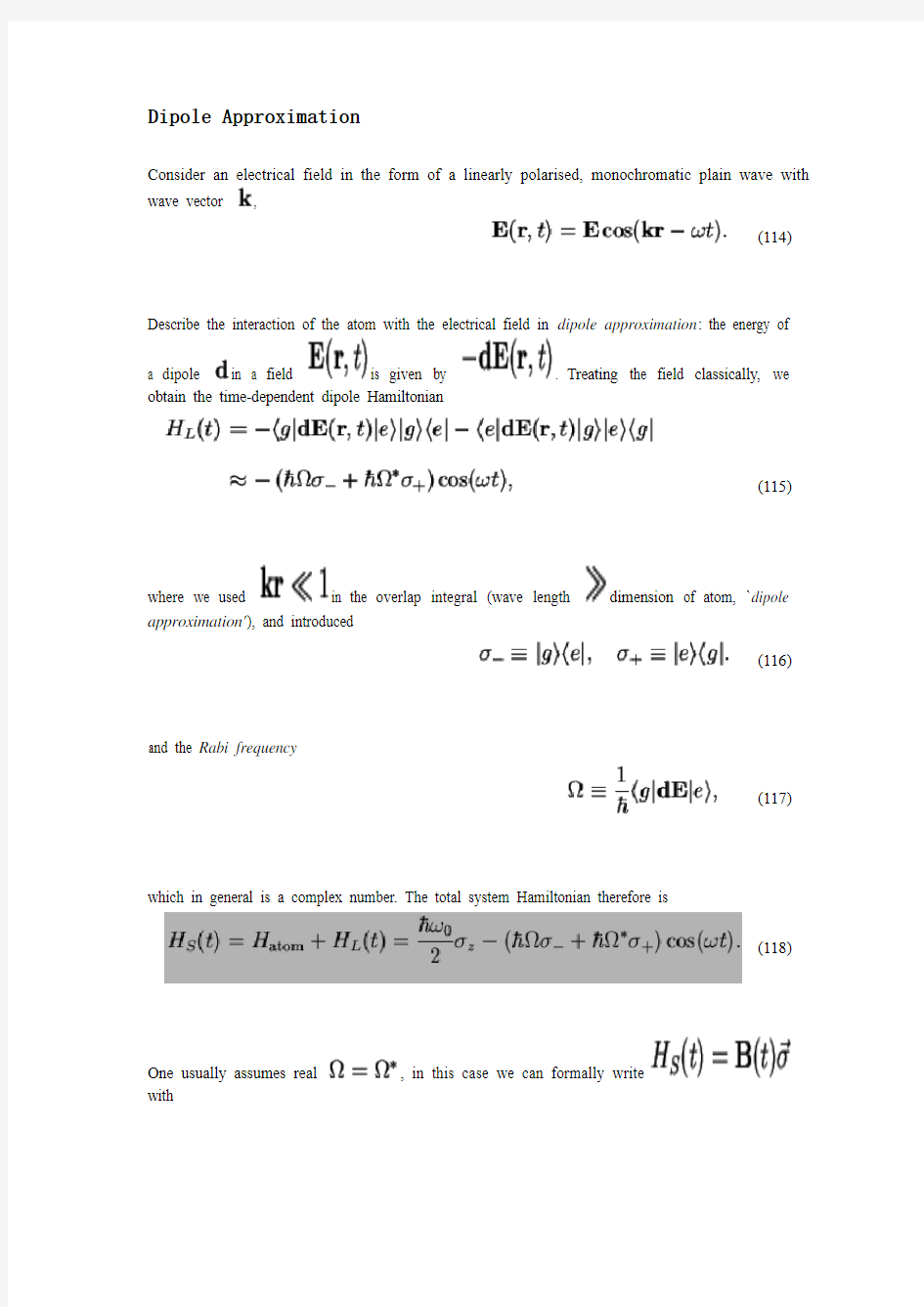
One usually assumes real , in this case we can formally write

with

(119)

补充：Expanded as a series, the exponential factor describing the x-ray radiation field at the

absorbing atom or molecule has the form

1 + O(k) + O(k2) + ...,

where k is the x-ray wave vector (2π/λ) and O(k n) comprises terms proportional to the nth power

of k. The dipole (or electric dipole) approximation refers to keeping only the 1, so it is also the

zeroth-order approximation.

MORE TROUBLE FOR THE DIPOLE APPROXIMATION

A multi-institutional collaboration comprising both theorists and experimentalists working at the ALS has made

measurements of second-order nondipole effects in the angular dependence of the cross section for neon valen The finding potentially applies to a wide variety of x-ray photoemission studies, including gas-phase, surface-s materials-science work, where researchers may now need to account for the influence of higher-order nondipole standard dipole approximation conventionally applied to the interaction of x rays with matter.

Expanded as a series, the exponential factor describing the

Finding the Devil x-ray radiation field at the absorbing atom or molecule has

the form

1 + O(k) + O(k 2) + ...,

where k is the x-ray wave vector (2π/λ) and O(k n ) comprises terms proportional to the nth power of k. The dipole (or electric dipole) approximation refers to keeping only the 1, so it is also the zeroth-order approximation.

Within the dipole approximation, the differential cross section (cross section per unit solid angle) for angle-resolved photoemission with linearly polarized x rays is described by three quantities: the partial cross section, σ(h ν), the angular-distribution parameter, β(h ν), and the angle (θ) of the photoelectron trajectory relative to the polarization vector. When extracted from angular distribution

measurements, σ(h ν) and β(h ν) provide information about the electronic structure of the atom and the molecule and the dynamics of the photoionization process. For example, at the "magic angle" θ = 54.7o, the angular term disappears and σ(h ν) is obtained.

In the dipole approximation, a single term

describes

electron

angular

distributions as a function of the angle θ relative to the polarization, E, of the radiation.

Higher-order

photon

interactions lead to nondipole effects, which in the experiments reported here can

be

described

by two

new

parameters and a second angle, φ, relative to the propagation direction, k, of the radiation.

in the Details

Scientists studying atoms and molecules use x rays to determine the "electronic structure" comprising the electron orbitals and their characteristics. Photoemission is a good example. From the spectrum of kinetic energies and directions of travel of photoelectrons emitted from the atom or molecule after absorbing x rays, investigators can work backwards to reconstruct the electronic structure. However, this process requires theoretical models that not only accurately describe the interaction of the x ray with the atom or molecule but that are also solvable in a practical way. For this reason, scientists use as much as possible a simplification of the x-ray interaction called the dipole approximation. However, in the last few years, scientists

conducting very careful measurements at the ALS and elsewhere have found that in surprising circumstances the dipole approximation is not sufficiently accurate. A more accurate approximation with extra "first-order" corrections helped but did not eliminate the discrepancies between theory and experiment in every case. Now a collaboration of theorists and experimentalists working at the ALS has both calculated the

effects of even more

sophisticated "second-order"

corrections and experimentally

verified their importance at

unexpectedly low energies.

Researchers in several fields

may now need to take these

nondipole effects into account.

It has long been known that this approximation is not valid for high photon energies (e.g., above 5 keV), where the photon wavelength is smaller than the size of the atom or molecule. In the last few years, groups working at the ALS and elsewhere have shown that additional first-order nondipole (specifically, electric quadrupole) terms are needed in the rare gases at lower photon energies and close to an ionization threshold. These terms involve two first-order energy-dependent parameters, δ(hν) and γ(hν), and a new angle variable (φ).

At this level of approximation, the recent rare-gas experiments showed significant modifications of the photoelectron angular distributions compared to those expected within the dipole approximation, modifications that were in generally good agreement with the first-order calculations. However, when conducting the analysis for neon in terms of the γ(hν) for 2s photoemission and ζ(hν) (where ζ = 3δ + γ) for 2p photoemission, experimenters at the ALS noticed that some discrepancy remained, particularly for neon 2p photoemission.

Theorists among the group calculated a general expression for the angle-resolved photoemission cross section including second-order contributions, which introduced four new energy-dependent nondipole factors dominated by electric-octupole and pure electric-quadrupole effects. Since no new angles were involved, the second-order corrections could then be recast in terms of effective values of γ(hν) and ζ(hν) for comparison with their measurements on neon.

The group made this comparison for four geometries, two with θ at the magic angle where only nondipole terms are important, and two on a "nondipole cone" at an angle of 35.3oaround the direction of the x-ray beam. Comparison of experiment with first-order theory yielded good agreement for both neon 2s and 2p photoemission for detectors on the nondipole cone, but in the magic-angle geometry, second-order corrections were needed, especially for neon 2p.

Experimental and theoretical values of the first-order

correction terms γ2s and ζ2p for neon 2s and 2p

photoemission determined in "magic-angle" and

"nondipole-cone" geometries.

The complex angular dependence of the differential cross section means that which corrections to the dipole approximation are needed depends on the experimental geometry, but the new results demonstrate that researchers need to be ready to include nondipole effects through at least the second order in analyzing their results.

Research conducted by A. Derevianko and W.R. Johnson (University of Notre Dame); O. Hemmers, S. Oblad, and D.W. Lindle (University of Nevada, Las Vegas); P. Glans (Stockholm University); H. Wang (Uppsala University); S.B. Whitfield (University of Wisconsin); R. Wehlitz (University of Wisconsin); and I.A. Sellin (University of Tennessee, Knoxville).

Research funding: National Science Foundation, EPSCoR Program of the U.S. Department of Energy, and University of Nevada, Las Vegas. Operation of the ALS is supported by the Office of Basic Energy Sciences, U.S. Department of Energy.

Publication about this experiment: A. Derevianko, O. Hemmers, S. Oblad, P. Glans, H. Wang, S.B.Whitfield, R. Wehlitz, I.A. Sellin, W.R. Johnson, and D.W. Lindle,

"Electric-Octupole and Pure-Electric-Quadrupole Effects in Soft-X-Ray Photoemission,"

Phys. Rev. Lett. 84, 2116 (2000).

ALSNews Vol. 170, February 14, 2001

The electric dipole approximation

In general, the wave-length of the type of electromagnetic radiation which induces, or is emitted during, transitions between different atomic energy levels is much larger than the typical size of a light atom. Thus,

(845)

can be approximated by its first term, unity (remember that ). This approximation is known as the electric dipole approximation. It follows that

(846) It is readily demonstrated that

(847) so

(848) Using Eq. (844), we obtain

(849)

where is the fine structure constant. It is clear that if the absorption cross-section is regarded as a function of the applied frequency, , then it exhibits a sharp maximum at

.

Suppose that the radiation is polarized in the -direction, so that . We have already seen, from Sect. 6.4, that

unless the initial and final states satisfy

(850)

(851)

Here, is the quantum number describing the total orbital angular

momentum of the electron, and is the quantum number describing the projection of the orbital angular momentum along the -axis. It is easily

demonstrated that and are only non-zero if

(852)

(853)

Thus, for generally directed radiation is only non-zero if

(854)

(855)

These are termed the selection rules for electric dipole transitions. It is clear, for instance, that the electric dipole approximation allows a transition from a

state to a state, but disallows a transition from a to a state. The

latter transition is called a forbidden transition.

Forbidden transitions are not strictly forbidden. Instead, they take place at a far lower rate than transitions which are allowed according to the electric dipole approximation. After electric dipole transitions, the next most likely type of transition is a magnetic dipole transition, which is due to the interaction between the electron spin and the oscillating magnetic field of the incident electromagnetic radiation. Magnetic dipole transitions are typically about times more

unlikely than similar electric dipole transitions. The first-order term in Eq. (845) yields so-called electric quadrupole transitions. These are typically about times more unlikely

than electric dipole transitions. Magnetic dipole and electric quadrupole transitions satisfy different selection rules than electric dipole transitions: for instance, the selection rules for

electric quadrupole transitions are . Thus, transitions which are forbidden as electric dipole transitions may well be allowed as magnetic dipole or electric quadrupole transitions.

Integrating Eq. (849) over all possible frequencies of the incident radiation yields

(856)

Suppose, for the sake of definiteness, that the incident radiation is polarized in the -direction. It is easily demonstrated that

(857) Thus,

(858) giving

(859) It follows that

(860) This is known as the Thomas-Reiche-Kuhn sum rule. According to this rule, Eq. (856) reduces to

(861)

Note that has dropped out of the final result. In fact, the above formula is

exactly the same as that obtained classically by treating the electron as an oscillator.

Electric Dipole Approximation and Selection Rules

We can now expand the term to allow us to

compute matrix elements more easily. Since and the matrix element is

squared, our expansion will be in powers of which is a small number. The dominant decays will be those from the zeroth order approximation which is

This is called the Electric dipole approximation.

In this Electric Dipole approximation, we can make general progress on computation of the matrix

element. If the Hamiltonian is of the form and

, then

and we can write in terms of the commutator.

This equation indicates the origin of the name Electric Dipole: the matrix element is of the vector which is a dipole.

We can proceed further, with the angular part of the (matrix element) integral.

At this point, lets bring all the terms in the formula back together so we know what we are doing.

We will attempt to clearly separate the terms due to for the sake of modularity of the calculation.

The integral with three spherical harmonics in each term looks a bit difficult, but, we can use a Clebsch-Gordan series like the one in addition of angular momentum to help us solve the problem. We will write the product of two spherical harmonics in terms of a sum of spherical

harmonics. Its very similar to adding the angular momentum from the two s. Its the same series as we had for addition of angular momentum (up to a constant). (Note that things

will be very simple if either the initial or the final state have , a case we will work out below for transitions to s states.) The general formula for rewriting the product of two spherical harmonics (which are functions of the same coordinates) is

The square root and can be thought of as a normalization constant in an

otherwise normal Clebsch-Gordan series. (Note that the normal addition of the orbital angular momenta of two particles would have product states of two spherical harmonics in different coordinates, the coordinates of particle one and of particle two.) (The derivation of the above equation involves a somewhat detailed study of the properties of rotation matrices and would take us pretty far off the current track (See Merzbacher page 396).)

First add the angular momentum from the initial state and the photon

using the Clebsch-Gordan series, with the usual notation for the Clebsch-Gordan

coefficients.

I remind you that the Clebsch-Gordan coefficients in these equations are just numbers which are less than one. They can often be shown to be zero if the angular momentum doesn't add up. The equation we derive can be used to give us a great deal of information.

We know, from the addition of angular momentum, that adding angular momentum 1 to

can only give answers in the range so the

change in in between the initial and final state can only be . For other values, all the Clebsch-Gordan coefficients above will be zero.

We also know that the are odd under parity so the other two spherical harmonics must

have opposite parity to each other implying that , therefore

We also know from the addition of angular momentum that the z components just add like integers, so the three Clebsch-Gordan coefficients allow

We can also easily note that we have no operators which can change the spin here. So certainly

We actually haven't yet included the interaction between the spin and the field in our calculation, but, it is a small effect compared to the Electric Dipole term.

The above selection rules apply only for the Electric Dipole (E1) approximation. Higher order terms in the expansion, like the Electric Quadrupole (E2) or the Magnetic Dipole (M1), allow other decays

but the rates are down by a factor of or more. There is one absolute selection rule coming

from angular momentum conservation, since the photon is spin 1. No to

transitions in any order of approximation.

As a summary of our calculations in the Electric Dipole approximation, lets write out the decay rate formula.