fluent欧拉离散模型算例
Chapter 23: Using the Eulerian Multiphase Model for Granular Flow This tutorial is divided into the following sections:
23.1. Introduction
23.2. Prerequisites
23.3. Problem Description
23.4. Setup and Solution
23.5. Summary
23.6. Further Improvements
23.1. Introduction
Mixing tanks are used to maintain solid particles or droplets of heavy fluids in suspension. Mixing may
be required to enhance reaction during chemical processing or to prevent sedimentation. In this tutorial, you will use the Eulerian multiphase model to solve the particle suspension problem.The Eulerian multiphase model solves momentum equations for each of the phases, which are allowed to mix in any proportion.
This tutorial demonstrates how to do the following:
?Use the granular Eulerian multiphase model.
?Specify fixed velocities with a user-defined function (UDF) to simulate an impeller.
?Set boundary conditions for internal flow.
?Calculate a solution using the pressure-based solver.
?Solve a time-accurate transient problem.
23.2. Prerequisites
This tutorial is written with the assumption that you have completed one or more of the introductory tutorials found in this manual:
?Introduction to Using ANSYS FLUENT in ANSYS Workbench: Fluid Flow and Heat Transfer in a Mixing Elbow (p.1)
?Parametric Analysis in ANSYS Workbench Using ANSYS FLUENT (p.77)
?Introduction to Using ANSYS FLUENT: Fluid Flow and Heat Transfer in a Mixing Elbow (p.131)
and that you are familiar with the ANSYS FLUENT navigation pane and menu structure. Some steps in
the setup and solution procedure will not be shown explicitly.
23.3. Problem Description
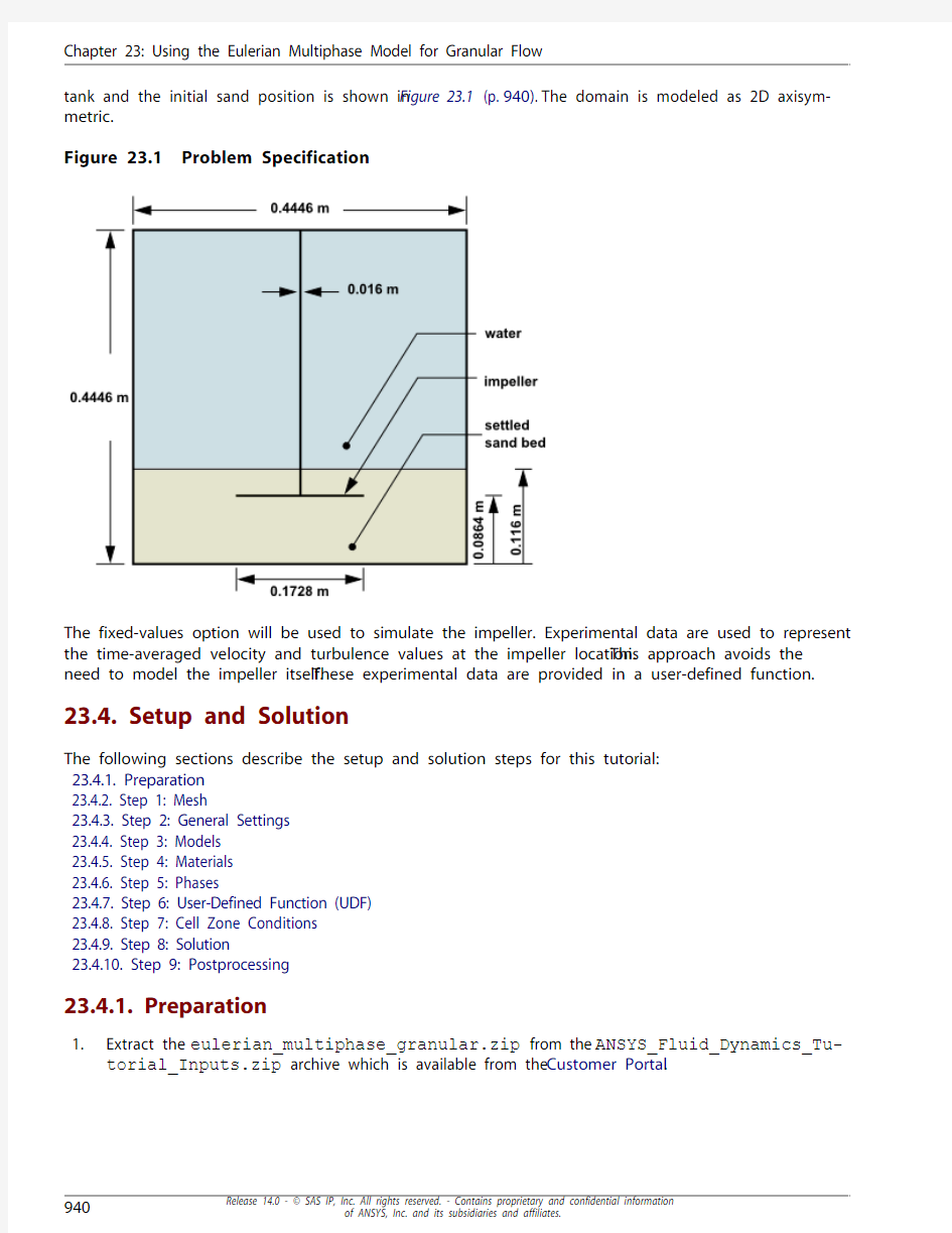
The problem involves the transient startup of an impeller-driven mixing tank.The primary phase is water, while the secondary phase consists of sand particles with a 111 micron diameter.The sand is initially settled at the bottom of the tank, to a level just above the impeller. A schematic of the mixing
Chapter 23: Using the Eulerian Multiphase Model for Granular Flow
tank and the initial sand position is shown in Figure 23.1 (p.940).The domain is modeled as 2D axisym-metric.
Figure 23.1 Problem Specification
The fixed-values option will be used to simulate the impeller. Experimental data are used to represent
the time-averaged velocity and turbulence values at the impeller location.This approach avoids the
need to model the impeller itself.These experimental data are provided in a user-defined function. 23.4. Setup and Solution
The following sections describe the setup and solution steps for this tutorial:
23.4.1. Preparation
23.4.2. Step 1: Mesh
23.4.3. Step 2: General Settings
23.4.4. Step 3: Models
23.4.5. Step 4: Materials
23.4.6. Step 5: Phases
23.4.7. Step 6: User-Defined Function (UDF)
23.4.8. Step 7: Cell Zone Conditions
23.4.9. Step 8: Solution
23.4.10. Step 9: Postprocessing
23.4.1. Preparation
1.Extract the eulerian_multiphase_granular.zip from the ANSYS_Fluid_Dynamics_Tu-
torial_Inputs.zip archive which is available from the Customer Portal.
Setup and Solution Note
For detailed instructions on how to obtain the ANSYS_Fluid_Dynamics_Tutori-
al_Inputs.zip file, please refer to Preparation (p.3) in Introduction to Using ANSYS
FLUENT in ANSYS Workbench: Fluid Flow and Heat Transfer in a Mixing Elbow (p.1).
2.Unzip eulerian_multiphase_granular.zip.
The files,mixtank.msh and fix.c can be found in the eulerian_multiphase_granular
folder created after unzipping the file.
https://www.360docs.net/doc/e418550713.html,e FLUENT Launcher to start the 2D version of ANSYS FLUENT.
4.Enable Double-Precision.
For more information about FLUENT Launcher, see Starting ANSYS FLUENT Using FLUENT Launcher in the User’s Guide.
Note
The Display Options are enabled by default.Therefore, after you read in the mesh, it will
be displayed in the embedded graphics window.
Note
The double precision solver is recommended for modeling multiphase flow simulations.
23.4.2. Step 1: Mesh
1.Read the mesh file mixtank.msh.
File?Read?Mesh...
A warning message will be displayed twice in the console.You need not take any action at this point,
as the issue will be rectified when you define the solver settings in Step 2.
23.4.3. Step 2: General Settings
General
1.Check the mesh.
General?Check
ANSYS FLUENT will perform various checks on the mesh and report the progress in the console. Ensure that the reported minimum volume is a positive number.
2.Examine the mesh (Figure 2
3.2 (p.942)).
Figure 23.2 Mesh Display
Extra
You can use the right mouse button to check which zone number corresponds to each boundary. If you click the right mouse button on one of the boundaries in the graphics window, its zone number, name, and type will be printed in the console.This feature is especially useful when you have several zones of the same type and you want to distinguish between them quickly.
3.
Modify the mesh colors.General ? Display...a.
Click the Colors... button to open the Mesh Colors dialog box.
Chapter 23: Using the Eulerian Multiphase Model for Granular Flow
Setup and Solution You can control the colors used to draw meshes by using the options available in the Mesh Colors dialog box.
i.Select Color by ID in the Options list.
This will assign a different color to each zone in the domain, rather than to each type of
zone.
ii.Close the Mesh Colors dialog box.
b.Click Display and close the Mesh Display dialog box.
The graphics display will be updated to show the mesh.
Chapter 23: Using the Eulerian Multiphase Model for Granular Flow
Figure 23.3 Mesh Display Using the C
olor by ID Option Array 4.Modify the view of the mesh display to show the full tank upright.
Graphics and Animations?Views...
Setup and Solution
a.Select axis from the Mirror Planes selection list and click Apply.
The mesh display will be updated to show both sides of the tank.
b.Click Auto Scale.
This option is used to scale and center the current display without changing its orientation (Figure
23.4 (p.946)).
Figure 23.4 Mesh Display of the Tank, Mirrored and Scaled
c.Click the Camera... button to open the Camera Parameters
dialog box.
Chapter 23: Using the Eulerian Multiphase Model for Granular Flow
Setup and Solution
i.Drag the indicator of the dial with the left mouse button in the counter-clockwise direction
until the upright view is displayed (Figure 23.5 (p.947)).
ii.Click Apply and close the Camera Parameters dialog box.
d.Close the Views dialog box.
Note
While modifying the view, you may accidentally lose the view of the geometry in the
display.You can easily revert to the default (front) view by clicking the Default button
in the Views dialog box.
Figure 23.5 Mesh Display of the Upright Tank
5.Specify a transient, axisymmetric model.
General
Chapter 23: Using the Eulerian Multiphase Model for Granular Flow
a.Retain the default Pressure-Based solver.
The pressure-based solver must be used for multiphase calculations.
b.Select Transient in the Time list.
c.Select Axisymmetric in the 2D Space list.
6.Set the gravitational acceleration.
a.Enable Gravity.
b.Enter -9.81 m/ for the Gravitational Acceleration in the X direction.
23.4.4. Step 3: Models
Models
1.Enable the Eulerian multiphase model.
Models?Multiphase?Edit...
a.Select Eulerian in the Model list.
b.Retain the default setting of 2 for Number of Eulerian Phases.
c.Click OK to close the Multiphase Model dialog box.
2.Enable the - turbulence model with standard wall functions.
Models?
Viscous?Edit...
Setup and Solution
a.Select k-epsilon (2eqn) in the Model list.
b.
Select Standard Wall Functions in the Near-Wall Treatment list.
This problem does not require a particularly fine mesh hence, standard wall functions can be used.
c.Select Dispersed in the Turbulence Multiphase Model list.
The dispersed turbulence model is applicable in this case because there is clearly one primary continuous phase and the material density ratio of the phases is approximately 2.5. Furthermore,the Stokes number is much less than 1.Therefore, the kinetic energy of the particle will not differ significantly from that of the liquid. For more information, see Model Comparisons in the Theory Guide.
d.Click OK to close the Viscous Model dialog box.
23.4.5. Step 4: Materials
Materials
In this step, you will add liquid water to the list of fluid materials by copying it from the ANSYS FLUENT ma-terials database and create a new material called sand.1.
Copy liquid water from the FLUENT materials database so that it can be used for the primary phase.
Chapter 23: Using the Eulerian Multiphase Model for Granular Flow
Setup and Solution
Materials?Fluid?Create/Edit...
dialog box.
a.Click the FLUENT Database... button to open the FLUENT Database Materials Array
b.Select water-liquid (h2o l ) from the FLUENT Fluid Materials selection list.
Scroll down the FLUENT Fluid Materials list to locate water-liquid (h2o l ).
c.Click Copy to copy the information for liquid water to your model.
d.Close the FLUENT Database Materials dialog box.
2.Create a new material called sand.
Chapter 23: Using the Eulerian Multiphase Model for Granular Flow
a.Enter sand for Name and delete the entry in the Chemical Formula field.
b.Enter 2500 kg/ for Density in the Properties group box.
c.Click Change/Create.
A Question dialog box will open, asking if you want to overwrite water-liquid.
d.Click No in the Question dialog box to retain water-liquid and add the new material (sand) to
the list.
The Create/Edit Materials dialog box will be updated to show the new material,sand, in the
FLUENT Fluid Materials drop-down list.
3.Close the Create/Edit Materials dialog box.
23.4.6. Step 5: Phases
Phases
Setup and Solution
1.Specify water (water-liquid ) as the primary phase.
Edit...
Phases?phase-1?
a.Enter water for Name.
b.Select water-liquid from the Phase Material drop-down list.
c.Click OK to close the Primary Phase dialog box.
2.Specify sand (sand ) as the secondary phase.
Phases?phase-2?Edit...
Chapter 23: Using the Eulerian Multiphase Model for Granular Flow
a.Enter sand for Name.
b.Select sand from the Phase Material drop-down list.
c.Enable Granular.
d.Retain the selection of Phase Property in the Granular Temperature Model list.
e.Enter 0.000111 m for Diameter.
f.Select syamlal-obrien from the Granular Viscosity drop-down list.
g.Select lun-et-al from the Granular Bulk Viscosity drop-down list.
h.Enter 0.6 for Packing Limit.
Scroll down in the Properties group box to locate Packing Limit.
i.Click OK to close the Secondary Phase dialog box.
3.Specify the drag law to be used for computing the interphase momentum transfer.
Phases?Interaction...
Setup and Solution
a.Select gidaspow from the Drag Coefficient drop-down list.
b.Click OK to close the Phase Interaction dialog box.
23.4.7. Step 6: User-Defined Function (UDF)
A UDF is used to specify the fixed velocities that simulate the impeller.The values of the time-averaged impeller velocity components and turbulence quantities are based on experimental measurement.The variation of these values may be expressed as a function of radius, and imposed as polynomials according to: =++++…
The order of polynomial to be used depends on the behavior of the function being fitted. For this tutorial,
the polynomial coefficients shown in Table 23.1: Impeller Profile Specifications (p.955)
Table 23.1 Impeller Profile Specifications
A1
A2
Variable
A3
A5
A6
A4
u velocity
-7.1357e-2
54.304
–
4.5578e+4
-1.966e+5
-3.1345e+3
3.1131e-2
v velocity
-10.313
–
1.186e+5
9.5558e+2
-2.0051e+4
kinetic energy
2.2723e-2
6.7989
1.8410e+5
9.4615e+3
-7.725e+4
-424.18
-6.5819e-2
dissipation
88.845
-9.120e+5
-5.3731e+3
1.1643e+5
1.9567e+6 For more information about setting up a UDF using the DEFINE_PROFILE macro, refer to the separate UDF Manual.Though this macro is usually used to specify a profile condition on a boundary face zone,
it is used in fix.c to specify the condition in a fluid cell zone. Hence, the arguments of the macro
have been changed accordingly.
1.Interpret the UDF source file fix.c.
Chapter 23: Using the Eulerian Multiphase Model for Granular Flow
Define?User-Defined?Functions?
Interpreted...
a.Enter fix.c for Source File Name.
If the UDF source file is not in your working folder, you must enter the entire folder path for Source File Name instead of just entering the file name. Alternatively, click Browse... and select fix.c in
the eulerian_multiphase_granular folder that was created after you unzipped the ori-
ginal file.
b.Enable Display Assembly Listing.
The Display Assembly Listing option displays the assembly language code in the console as the
function compiles.
c.Click Interpret to interpret the UDF.
d.Close the Interpreted UDFs dialog box.
Note
The name and contents of the UDF are stored in the case file when you save the
case file.
23.4.8. Step 7: Cell Zone Conditions
Cell Zone Conditions
Setup and Solution
For this problem, you do not have to specify any conditions for outer boundaries.Within the domain, there
are three fluid zones, representing the impeller region, the region where the sand is initially located, and the rest of the tank.There are no conditions to be specified in the latter two zones, so you need to set conditions only in the zone representing the impeller.
1.Set the boundary conditions for the fluid zone representing the impeller (fix-zone) for the primary
phase.
Cell Zone Conditions?fix-zone
You will specify the conditions for water and sand separately using the UDF.The default conditions
for the mixture (i.e., conditions that apply to all phases) are acceptable.
a.Select fix-zone in the Zone list.
b.Select water from the Phase drop-down list.
c.Click the Edit... button to open the Fluid dialog box.
i.Enable Fixed Values .
The Fluid dialog box will expand to show the related inputs.
ii.Click the Fixed Values tab and set the following fixed values:
Value Parameter
udf fixed_u Axial Velocity udf fixed_v Radial Velocity udf
fixed_ke Turbulence Kinetic En-ergy
udf
fixed_diss
Turbulence Dissipation Rate
d.Click OK to close the Fluid dialog box.
2.
Set the boundary conditions for the fluid zone representing the impeller (fix-zone ) for the secondary phase.
Cell Zone Conditions ? fix-zone
a.Make sure that fix-zone is selected in the Type list.
b.Select sand from the Phase drop-down list.
c.
Click the Edit... button to open the Fluid dialog box.
Chapter 23: Using the Eulerian Multiphase Model for Granular Flow