美赛论文优秀模版可编辑

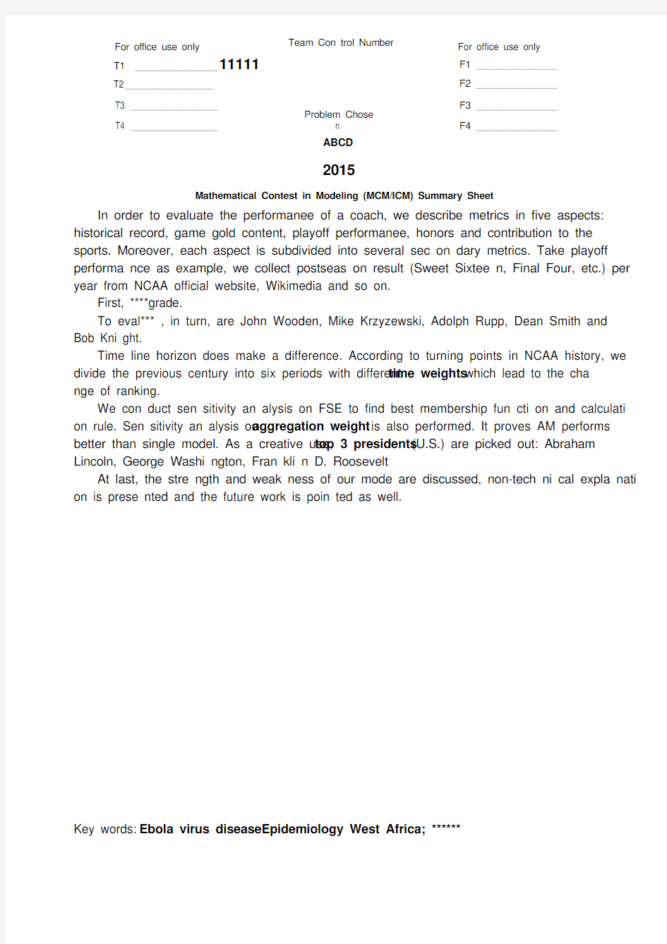
Team Con trol Number

For office use only

2015

Mathematical Contest in Modeling (MCM/ICM) Summary Sheet

In order to evaluate the performanee of a coach, we describe metrics in five aspects:

historical record, game gold content, playoff performanee, honors and contribution to the sports. Moreover, each aspect is subdivided into several sec on dary metrics. Take playoff performa nce as example, we collect postseas on result (Sweet Sixtee n, Final Four, etc.) per year from NCAA official website, Wikimedia and so on.

First, ****grade.

To eval*** , in turn, are John Wooden, Mike Krzyzewski, Adolph Rupp, Dean Smith and Bob Kni ght.

Time line horizon does make a difference. According to turning points in NCAA history, we divide the previous century into six periods with different time weights which lead to the cha nge of ranking.

We con duct sen sitivity an alysis on FSE to find best membership fun cti on and calculati on rule. Sen sitivity an alysis on aggregation weight is also performed. It proves AM performs better than single model. As a creative use,top 3 presidents (U.S.) are picked out: Abraham Lincoln, George Washi ngton, Fran kli n D. Roosevelt

At last, the stre ngth and weak ness of our mode are discussed, non-tech ni cal expla nati on is prese nted and the future work is poin ted as well.

Key words: Ebola virus diseaseEpidemiology West Africa; ******

T1 _______________ 11111

T2 ________________

F1 _______________ F2 _______________ T3 ________________

T4 ________________ Problem Chose

n ABCD

F3 _______________ F4 _______________

For office use only

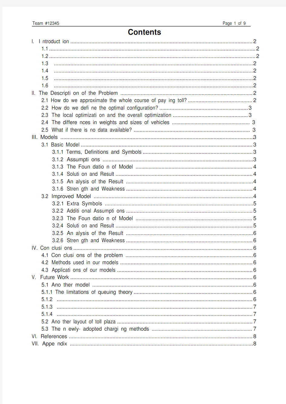
Contents

I. I ntroduct ion (2)

1.1 (2)

1.2 (2)

1.3 (2)

1.4 (2)

1.5 (2)

1.6 (2)

II. The Descripti on of the Problem (2)

2.1 How do we approximate the whole course of pay ing toll? (2)

2.2 How do we defi ne the optimal configuration? (3)

2.3 The local optimizati on and the overall optimization (3)

2.4 The differe nces in weights and sizes of vehicles (3)

2.5 What if there is no data available? (3)

III. Models (3)

3.1 Basic Model (3)

3.1.1 Terms, Definitions and Symbols (3)

3.1.2 Assumpti ons (3)

3.1.3 The Foun datio n of Model (4)

3.1.4 Soluti on and Result (4)

3.1.5 An alysis of the Result (4)

3.1.6 Stren gth and Weakness (4)

3.2 Improved Model (4)

3.2.1 Extra Symbols (5)

3.2.2 Additi onal Assumpti ons (5)

3.2.3 The Foun datio n of Model (5)

3.2.4 Soluti on and Result (5)

3.2.5 An alysis of the Result (6)

3.2.6 Stren gth and Weakness (6)

IV. Con clusi ons (6)

4.1 Con clusi ons of the problem (6)

4.2 Methods used in our models (6)

4.3 Applicati ons of our models (6)

V. Future Work (6)

5.1 Ano ther model (6)

5.1.1 The limitations of queuing theory (6)

5.1.2 (6)

5.1.3 (7)

5.1.4 (7)

5.2 Ano ther layout of toll plaza (7)

5.3 The n ewly- adopted chargi ng methods (7)

VI. References (8)

VII. Appe ndix (8)

I. I ntroduction

In order to indicate the origin of the toll way problems, the following background is worth men ti oning.

1.1

1.2

1.3

1.4

1.5

1.6

II. The Description of the Problem

2.1 How d o we approximate the whole course of pay ing toll?

2.2 How d o we defi ne the optimal con figurati on?

1) From the perspective of motorist:

2) From the perspective of the toll plaza:

3) Compromise:

2.3 The l ocal optimization and the overall optimization

Virtually:

2.4 The differe nces in weights and sizes of vehicl es

2.5 What if there is no data availabl e?

III. Models

3.1 Basic Model

3.1.1 Terms, Definitions and Symbols

The sig ns and defi niti ons are mostly gen erated fronqueu ing theory.

3.1.2 Assumpti ons

3.1.3 The Foun dation of Model

1) The utility function

The cost of toll plaza:

The loss of motorist:

The weight of each aspect:

Compromise:

2) The integer programming

Accord ing to queu ing theory, we can calculate the statistical properties as follows.

3) The overall optimization and the local optimization

The overall optimization:

The local optimization:

The optimal number of tollbooths:

3.1.4 Solution and Result

1) The solution of the integer programming:

2) Results:

3.1.5 An alysis of the Result

Local optimization and overalloptimization:

Sensitivity: The result is quite sen sitive to the cha nge of thehree parameters

Trend:

Comparison:

3.1.6 Stre ngth and Weak ness

Strength: In despite of this, the model has provedhat . Moreover, we have draw n

some useful con clusi on sabout . The model is fit for, such as

Weakness:This model just applies to . As we havestated, . That' s just what

we should do in the improved model.

3.2 Improved Model

3.2.1 Extra Symbols

Signs and defi niti ons in dicated above are still valid. Here are some extra sig ns and defi niti ons.

3.2.2 Additi onal Assumpti ons

Assumpti ons concerning the an terior process are the same as the Basic Model.

3.2.3 The Foun dation of Model

1) How do we determine the optimal number?

As we have con cluded from the Basic Model,

3.2.4 Solution and Result

1) Simulation algorithm

Based on the analysis above, we design our simulation arithmetic as follows.

Step1:

Step2:

Step3:

Step4:

Step5:

Step6:

Step7:

Step8:

Step9:

2) Flow chart

The figure below is the flow chart of the simulatio n.

3) Solution

3.2.5 Analysis of the Result

3.2.6 Stre ngth and Weak ness

Strength: The Improved Model aims to make up forthe n eglect of . The result seems to declare that this model is more reas on able tha n the Basic Model and much more effective tha n the existi ng desig n.

Weakness: . Thus the model is still an approximate on a large scale. This has

doomed to limit the applications of it.

IV. Conclusions

4.1 Con clusi ons of the

probl

4.2 Methods used in our mod els

4.3 Applicati ons of our

els

mod

V. Future Work

5.1 Ano ther

model

5.1.1 The limitations of queuing theory

5.1.2