Klobuchar-Ionospheric-Model
Klobuchar Ionospheric Model
GPS satellites broadcast the parameters of the Klobuchar ionospheric model for single frequency users. The Klobuchar model was designed to minimise user computational complexity and user computer storage as far as to keep a minimum number of coefficients to transmit on satellite-user link.
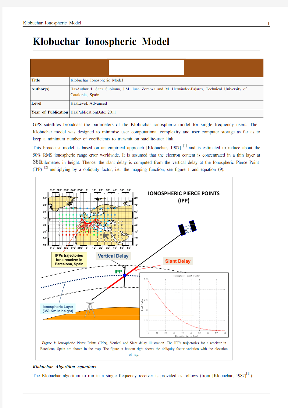
This broadcast model is based on an empirical approach [Klobuchar, 1987] [1] and is estimated to reduce about the 50% RMS ionospheric range error worldwide. It is assumed that the electron content is concentrated in a thin layer at kilometres in height. Thence, the slant delay is computed from the vertical delay at the Ionospheric Pierce Point (IPP) [2] multiplying by a obliquity factor, i.e., the mapping function, see figure 1 and equation (9).
Figure 1: Ionospheric Pierce Points (IPPs), Vertical and Slant delay illustration. The IPP's trajectories for a receiver in
Barcelona, Spain are shown in the map. The figure at bottom right shows the obliquity factor variation with the elevation
of ray.
Klobuchar Algorithm equations
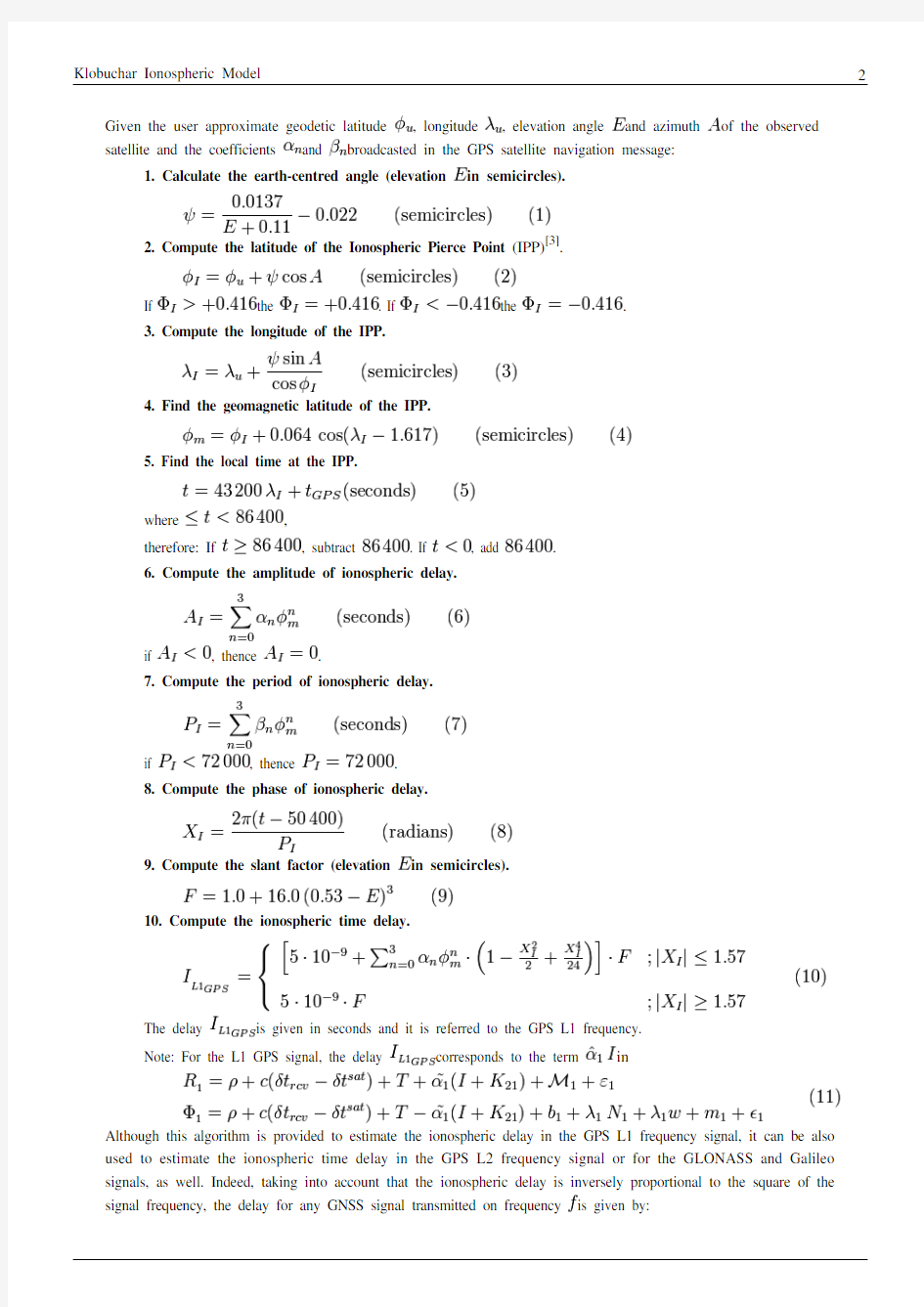
The Klobuchar algorithm to run in a single frequency receiver is provided as follows (from [Klobuchar, 1987][1]):
Given the user approximate geodetic latitude , longitude , elevation angle and azimuth of the observed satellite and the coefficients and broadcasted in the GPS satellite navigation message:
1. Calculate the earth-centred angle (elevation in semicircles).
2. Compute the latitude of the Ionospheric Pierce Point (IPP)[3].
If the . If the .
3. Compute the longitude of the IPP.
4. Find the geomagnetic latitude of the IPP.
5. Find the local time at the IPP.
where ,
therefore: If , subtract . If , add .
6. Compute the amplitude of ionospheric delay.
if , thence .
7. Compute the period of ionospheric delay.
if , thence .
8. Compute the phase of ionospheric delay.
9. Compute the slant factor (elevation in semicircles).
10. Compute the ionospheric time delay.
The delay is given in seconds and it is referred to the GPS L1 frequency.
Note: For the L1 GPS signal, the delay corresponds to the term in
Although this algorithm is provided to estimate the ionospheric delay in the GPS L1 frequency signal, it can be also used to estimate the ionospheric time delay in the GPS L2 frequency signal or for the GLONASS and Galileo signals, as well. Indeed, taking into account that the ionospheric delay is inversely proportional to the square of the
signal frequency, the delay for any GNSS signal transmitted on frequency is given by:
Figure 2 is a layout of the Klobuchar model algorithm, showing that the vertical delays are based on a constant value at night time and a half-cosine function in daytime, which amplitude and period are given as a function of the eight parameters ( ) broadcast in the GPS navigation message. A map with the geographical variation of the vertical delay is also depicted in this figure.
Figure 3 illustrates with an example the values of the GPS delays from the Klobuchar model and shows the effect of neglecting such delays in single point positioning for the horizontal and vertical error components.
Figure 2: Klobuchar ionospheric model. Algorithm layout.
Figure 3: Ionospheric correction: Range and position domain effect
First row shows the horizontal (left) and vertical (right) positioning error
using (blue) or not using (red) the Klobuchar ionospheric correction defined
in 1. The variation in range is shown in the second row at left
Notes
[1][Klobuchar, 1987] Klobuchar, J., 1987. Ionospheric Time-Delay Algorithms for Single-Frequency GPS Users. IEEE Transactions on
Aerospace and Electronic Systems (3), pp. 325-331.
[2]That is the intersection of the ray with the ionospheric layer at UNIQ-math-0-236579b4aa0058fc-QINU kilometres in height.
[3]That is, the latitude of the earth projection of the ionospheric intersection point with a mean ionospheric height layer at
UNIQ-math-1-236579b4aa0058fc-QINU kilometres.
References
Article Sources and Contributors5 Article Sources and Contributors
Klobuchar Ionospheric Model Source: https://www.360docs.net/doc/0918825371.html,/index.php?oldid=11615 Contributors: Carlos.Lopez, Jaume.Sanz
Image Sources, Licenses and Contributors
File:Fundamentals_Name.png Source: https://www.360docs.net/doc/0918825371.html,/index.php?title=File:Fundamentals_Name.png License: unknown Contributors: Timo.Kouwenhoven
File:Klobuchar_ IPP_slide.png Source: https://www.360docs.net/doc/0918825371.html,/index.php?title=File:Klobuchar_IPP_slide.png License: unknown Contributors: Carlos.Lopez
File:Klobuchar_Klobychar_slide.png Source: https://www.360docs.net/doc/0918825371.html,/index.php?title=File:Klobuchar_Klobychar_slide.png License: unknown Contributors: Carlos.Lopez
File:Klobuchar_H_Nov_ion.png Source: https://www.360docs.net/doc/0918825371.html,/index.php?title=File:Klobuchar_H_Nov_ion.png License: unknown Contributors: Carlos.Lopez
File:Klobuchar_V_Nov_ion.png Source: https://www.360docs.net/doc/0918825371.html,/index.php?title=File:Klobuchar_V_Nov_ion.png License: unknown Contributors: Carlos.Lopez
File:Klobuchar_Nov_iono_cor.png Source: https://www.360docs.net/doc/0918825371.html,/index.php?title=File:Klobuchar_Nov_iono_cor.png License: unknown Contributors: Carlos.Lopez