Measurement of Arcminute Scale Anisotropy with the BIMA Array

a r

X

i

v

:a

s t

r o

-

p

h

/

2

6

1

2v

2

2

6

S

e p

2

2

Submitted to Astrophysical Journal Measurement of Arcminute Scale Cosmic Microwave Background Anisotropy with the BIMA Array K.S.Dawson 1,W.L.Holzapfel 1,J.E.Carlstrom 2,3,M.Joy 4,https://www.360docs.net/doc/5e17798753.html,Roque 2,https://www.360docs.net/doc/5e17798753.html,ler 2,5and D.Nagai 2kdawson@https://www.360docs.net/doc/5e17798753.html, ABSTRACT We report the results of our continued study of arcminute scale anisotropy in the Cosmic Microwave Background (CMB)with the Berkeley-Illinois-Maryland Association (BIMA)array.The survey consists of ten independent ?elds selected for low infrared dust emission and lack of bright radio point sources.With obser-vations from the Very Large Array (VLA)at 4.8GHz,we have identi?ed point sources which could act as contaminants in estimates of the CMB power spec-trum and removed them in the analysis.Modeling the observed power spectrum with a single ?at band power with average multipole of ?eff =6864,we ?nd ?T =14.2+4.8?6.0μK at 68%con?dence.The signal in the visibility data exceeds the expected contribution from instrumental noise with 96.5%con?dence.We have also divided the data into two bins corresponding to di?erent spatial res-olutions in the power spectrum.We ?nd ?T 1=16.6+5.3?5.9μK at 68%con?dence for CMB ?at band power described by an average multipole of ?eff =5237and

?T 2<26.5μK at 95%con?dence for ?eff =8748.

Subject headings:cosmology:observation –cosmic microwave background

1.Introduction

Fluctuations in the distribution of matter at the epoch of recombination create large angular scale anisotropy in the Cosmic Microwave Background(CMB).This primordial anisotropy has been studied extensively at degree and sub-degree angular scales in order to place constraints on the parameters of cosmological models(Halverson et al.2002,de Bernardis et al.2002,Scott et al.2002,Lee et al.2001,Miller et al.2002,Padin et al. 2001).At arcminute scales,the primordial anisotropy is damped to negligible amplitude due to photon di?usion and the?nite thickness of the last scattering surface(Hu&White1997). On these smaller scales,secondary anisotropies such as the Sunyaev-Zeldovich e?ect(SZE) are expected to dominate the signal of the CMB power spectrum(Haiman&Knox1999). Studies of secondary anisotropy in the CMB have the potential to be a powerful probe of the growth of structure in the Universe.

In this paper,we report results from an ongoing program using the Berkeley-Illinois-Maryland Association(BIMA)interferometer to search for arcminute-scale CMB anisotropy. Discussion of the instrument,data reduction,expected signals(from both primary and sec-ondary anisotropies)and previous measurements is included in earlier publications(Holzapfel et al.2000and Dawson et al.2001,hereafter H2000and D2001respectively).We describe observations and criteria for?eld selection in§2.The Bayesian likelihood analysis used to constrain the CMB anisotropy is described in§3.The results are presented in§4including a discussion of tests for systematic errors in the analysis.Finally,in§5,we present the conclusion and comparison to simulations of the SZE.

2.Observations

Analysis of eleven?elds observed with the BIMA array during the summers of1997, 1998,and2000revealed a signi?cant detection of excess power(D2001).In an e?ort to achieve uniform sensitivity and selection criteria across our sample,we continued the project in the summer of2001with a subset of eight?elds from the original survey.Two new?elds were also added to the survey for a total of ten.Each?eld was observed with the BIMA array and the Very Large Array(VLA)6.

2.1.Field Selection

The two new?elds added to the survey,BDF12and BDF13,lie at Right Ascensions convenient for summer observations and outside of the galactic plane.This makes for a total of ten independent?elds for the survey in2001,covering approximately0.1square degrees. The?elds were selected from the IRAS100μm and VLA NVSS(Condon et al.1998)radio surveys to lie in regions with low dust contrast and no bright radio sources.In addition,we used SkyView to access digitized sky survey and ROSAT images to check for bright optical or x-ray emission which could complicate follow-up observations.The pointing centers for each of the ten?elds are given in Table1.

Two of the?elds used in the D2001analysis,PC1643+46and VLA1312+32,were originally selected to follow-up previously reported microwave decrements(Jones et al.1997; Richards et al.1997).A third?eld,in the direction of the high redshift quasar PSS0030+17, was originally selected as a distant cluster candidate.These three?elds did not follow the same selection criteria as the rest of the?elds and are not included in the present sample. Since observations of these?elds are not as deep as those for the other blank?elds,removing them from the survey does not have a signi?cant e?ect on the results reported in this paper.

2.2.BIMA Observations

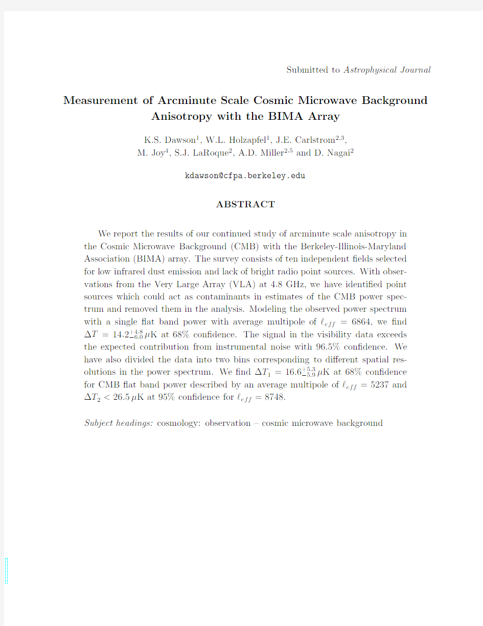
A priority for2001observations was to achieve uniform?ux sensitivity across the sample of ten?elds.We re-observed?elds from the previous years and dedicated55hours to each of the new?elds,aiming for a uniform noise level of<150μJy/beam RMS on short baselines (u-v<1.1kλ)for each?eld in the sample.This noise level corresponds to～15μK RMS for a2′synthesized beam.An image of the?eld BDF13observed with the BIMA array is included in Figure1to illustrate the sensitivity in the u-v range0.63?1.1kλ.

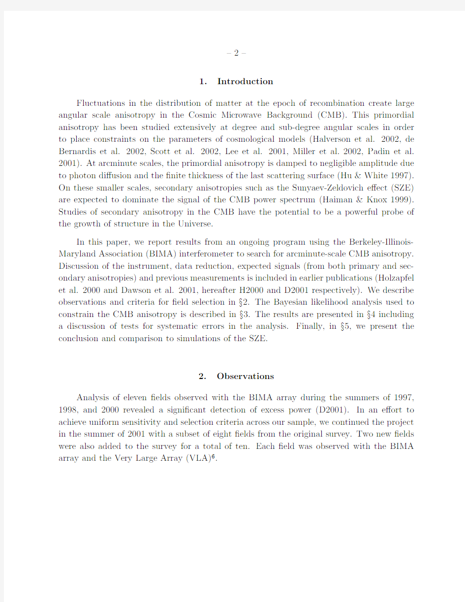
All anisotropy observations were made using the BIMA array at Hat Creek.Nine6.1 meter telescopes of the array were equipped for operation at28.5GHz,providing a6.6′FWHM?eld of view.In order to track phase and gain?uctuations,all?eld observations were bracketed by observations of bright radio point sources(H2000).The?uxes of these calibration sources are all referenced to the?ux of Mars which is uncertain by approximately 4%at90%con?dence(see discussion in Grego2001).This uncertainty is small compared to the uncertainty in the anisotropy signals we report here and therefore makes a negligible contribution to the uncertainties in the reported results.The cumulative integration time for each of the ten?elds observed in this survey is listed in Table1.Figure2shows the result of imaging the?eld BDF13using all of the u-v data from the summer of2001.This

image is a fair representation of the?elds in the survey which typically have only u-v data in the range0.63?3.0kλ.After calibration and data edits,a total of607hours of integration have been dedicated to this project.

2.3.VLA Observations and Point Source Results

Sources of foreground emission have the potential to contaminate estimates of the CMB power spectrum.Contaminants at28.5GHz arising from galactic sources such as dust, synchrotron,and free-free emission are expected to be below theμK level at arcminute angular scales in the regions of the sky selected for this survey.However,emission from radio point sources could contribute signi?cantly to excess power in the observations described here (e.g.Tegmark et al.2000).

The compact con?guration used for the BIMA anisotropy observations was designed to produce high sensitivity to extended sources.However,this con?guration has limited sensitivity on the long baselines which in principle could be used to locate and remove point sources.To help constrain the contribution from point sources to the anisotropy measurements,we used the VLA at a frequency of4.8GHz to observe each?eld in the survey.With1.5hours per?eld,these observations yielded an RMS?ux of～25μJy/beam for a9′FWHM region with the same pointing center as a BIMA?eld.The positions of all point sources with?ux>6σwithin8′of the pointing center have been recorded.Measured point sources with?uxes corrected for attenuation from the primary beam at4.8GHz are listed in Table2.An image of the?eld BDF13is shown in Figure3as an example of observations used to identify point sources from the VLA data.

If the spectra of the point sources are relatively?at or falling,deep observations with the VLA will identify those that lie near the noise level in the28.5GHz maps.However,it is possible that a radio source with a steeply inverted spectrum may lie below the VLA de-tection threshold but still contribute to the observations at28.5GHz.Advection dominated accretion?ows are thought to be the most common inverted spectrum sources.They typi-cally have a slowly rising spectrum,with a spectral index of0.3to0.4(Perna and DiMatteo, 2000).Such a shallow spectrum would only provide a factor of two increase in?ux between 4.8GHz and28.5GHz.

3.Analysis

The analysis in this paper is similar to that used to produce the previous BIMA anisotropy results and is based on the formalism presented in White et al.(1999)for the determination of the CMB power spectrum from interferometer data.We bin the visibility data and calculate joint con?dence intervals as described in H2000.The likelihood function to test a theory for a set of bandpowers,{C?},with n measured visibilities is de?ned

1

L({C?})=

?T d x?T(x)A(x)e2πi u·x,(3) where?T(x)is the temperature distribution on the sky,A(x)is the primary beam of the telescope,

?Bν

hc 2x4e x

= ?Bν

2π ?Bνw W ij(w),(7)

where

T2CMB

?T2≡

ηA 21

for each baseline.The reducedχ2is calculated from each visibility,j,recorded from a given baseline

χ2= j V?(u j)V(u j)

χ2.The noise correlation

matrix is calculated from the rescaled noise for each baseline as in H2000,C N ii=1

Although some?elds were observed in1998with longer baselines,most?elds in this survey were observed from the compact con?guration.The compact con?guration of the BIMA array was contained within a u-v radius of3.0kλ.These baselines are included in order to achieve a reasonable level of discrimination between the signature of a point source and the CMB anisotropy described in§3.1.In this manner,we remove the contribution to the measured power from linear combinations of baselines that may be corrupted by point source emission.With each additional point source constraint,a degree of freedom is lost and the uncertainty in the measured power increases accordingly.

4.Results

We have produced and analyzed images for each of the observed?elds.The statistics of the images are described in Table3(0.63?1.7kλ),4(0.63?1.1kλ),and5(1.1?1.7kλ). The reported RMS values are those expected from the noise properties of the visibilities. The RMS temperature measurement corresponds to the synthesized beamsize for the given uv coverage.The baselines used to produce the image statistics are the same as the baselines included in the two bins of visibility data for the CMB anisotropy analysis.The window function produced from the noise weighted sum of the window functions for the individual visibilities in the u-v range0.63?1.1kλhas an average value of?eff=5237with FWHM ?=2870.The window function for visibilities in the u-v range1.1?1.7kλhas an average value?eff=8748with FWHM?=4150.For the analysis using a single bin of data in the u-v range0.63?1.7kλ,?eff=6864with FWHM?=6800.The window functions for all three bands are plotted as a function of multipole in Figure4.

4.1.Measurement of Anisotropy

We present the results of the analysis of the BIMA data assuming a CMB power spec-trum that is described by one or two?at band powers.In Tables3,4,and5,we show the most likely?T with con?dence intervals for each of the ten?elds included in this survey. Results for the joint likelihood for all the data are also included.Figure5shows the rela-tive likelihoods as a function of assumed?T for a combined likelihood analysis of the ten ?elds.The results are normalized to unity likelihood for the case of no anisotropy signal. The measured signal exceeds that expected from instrument noise with97.8%con?dence for data which falls in the u-v range0.63?1.1kλand with96.5%con?dence for the single bin of visibility data that covers the u-v range0.63?1.7kλ.

We include a contour plot of the two dimensional likelihood function in Figure 6in order to demonstrate the correlation between the two ?at band power bins.Contours represent 68%,95%,and 99%con?dence intervals.We calculate the correlation between the two bandpower bins directly from the likelihood function,

F = (?T 1??T 1)(?T 2??T 2)(?T 1??T 2)2

(14)F = 3.738×10?111.448×10?11

1.448×10?111.920×10?10 (μK )

2.(15)

This matrix can be diagonalized with eigenvalues

F ′= 3.604×10?11001.933×10?10 (μK )2,(16)

and corresponding eigenvectors,X ′

1=0.996X 1+0.0893X 2and X ′

2=0.0893X 1?0.996X 2.

There is less than 10%correlation between the two bins of visibility data.

4.2.Systematics Check

We performed tests for systematic errors in all ?elds with signi?cant excess power as described in D2001.Due to ?nite computing resources,the analysis is limited to visibility data in u -v range 0.63?1.1k λdescribed by ?T 1.The power in the second bin is ?xed at ?T 2=0for all tests described in this section.We tested for sources of contamination that change with time.Assuming that a terrestrial source,the sun,or the moon varies in position by several degrees over the course of a few days,such a local e?ect should be discovered from analysis of subsets divided into hours of observation or days of observation described in D2001.For the ?eld BDF12,an analysis of three subsets divided into time of observation

and three subsets of date of observation revealed a range of values ?T 1=16.2+21.4?16.2μK to

?T 1=71.0+33.5?28.0μK,in each case consistent with the reported value of ?T 1=44.2+16.4?13.7μK.

For the ?eld BDF13,the various subsets were found to have most likely values in the range

?T 1=33.8μK to ?T 1=58.9μK,consistent with the reported value of ?T 1=38.8+17.2?15.9μK.

There was no signi?cant di?erence in the measured power in subsets divided by day of observation or in the subsets divided by hour of observation.

We also added three additional tests this year to search for systematic errors in BDF12and BDF13.We performed a jack-knife systematic test by breaking the data into subsets of four and ?ve telescopes looking for antenna based systematic errors.For a test of baseline

based systematic errors,we created an east-west baseline subset and a north-south baseline

subset.Subsets for BDF12had most likely values in the range?T1=30.7μK to?T1= 53.0μK while subsets for BDF13had most likely values in the range?T1=37.2μK to ?T1=41.9μK.There was approximately the same level of excess power in each subset,as well as all of the subsets described in D2001.The third test combined the raw visibilities from observations of several di?erent?elds taken in a single summer to look for correlations between observations of independent?elds.As would be expected for uncorrelated data,the analysis of the combined data sets revealed a measurement of excess power that is consistent with instrumental noise to68%con?dence.Overall,we?nd no evidence that our results are biased by systematic e?ects.

As discussed in§2.3,we have adopted a VLA?ux density limit of6σfor identifying point sources.We now consider how di?erent point source?ux density limits a?ect our estimates of CMB anisotropy.We test the e?ect of four di?erent point source models on the determination of the most likely?T1and con?dence intervals.The results are found in Table6.There is no signi?cant di?erence in the?T1determined from the range of models considered.As in D2001,the?at band power results are insensitive to the details of the point source analysis.

5.Conclusion

Over the course of three summers,we have used the BIMA array in a compact con?gura-tion at28.5GHz to search for CMB anisotropy in ten independent6.6′FWHM?elds.With these observations,we have detected arcminute scale anisotropy at better than95%con?-dence.In the context of an assumed?at band power model for the CMB power spectrum, we?nd?T=14.2+4.8

?6.0μK at68.3%con?dence with sensitivity on scales that correspond to an average harmonic multipole?eff=6864.We also present results after dividing the

visibility data into two bins of di?erent spatial resolution.We?nd?T1=16.6+5.3

?5.9μK at 68.3%con?dence on scales corresponding to an average harmonic multipole?eff=5237and ?T2<26.5μK at95%con?dence at?eff=8748.The results of the VLA observations appear to exclude the possibility of point source contamination and there is no indication of an obvious systematic error that would bias the observations.

Mason et al.(2002)have also reported a detection of excess power at somewhat larger

angular scales.They?nd?T=22.5+2.5

?3.6μK for data in the range2010

If the signal observed in the BIMA?elds is indeed caused by CMB anisotropy,there are a host of possible sources for excess power such as primary anisotropy,thermal SZE, kinetic SZE,patchy reionization,and the Ostriker-Vishniac e?ect.Of these candidates for CMB anisotropy,the thermal SZE from clusters of galaxies is expected to dominate on the scales where the BIMA instrument is most sensitive(see for example,Gnedin&Ja?e2001). Analytic models and simulations of cluster formation predict?T values that range from 4.3μK to15.0μK on angular scales of approximately two arcminutes.Figure7compares the results of this paper to the theoretical models.

The non-Gaussian characteristics of the CMB power spectrum caused by the thermal SZE may increase the uncertainty in measurements of the power spectrum due to sample variance.Current models suggest that these e?ects increase the uncertainty by a factor of 3over what is expected for the sample variance of a Gaussian distributed signal at?～5000(White,Hernquist,&Springel2002).Based on this argument,the e?ect of non-Gaussian sample variance contributes a standard deviation of3×

2/N?T is the sample variance in a Gaussian distributed signal. The uncertainty due to sample variance is approximately equal to the statistical uncertainty reported in this paper,increasing the overall uncertainty by40%,in agreement with the predictions of Zhang,Pen&Wang(2002).The predicted e?ect of sample variance on the measurements is represented by the extended error bars in Figure7.

We thank the entire sta?of the BIMA observatory for their many contributions to this project,in particular Rick Forster and Dick Plambeck for their assistance with both the instrumentation and observations.Nils Halverson and Martin White are thanked for stimulating discussions concerning data analysis.We are grateful for the scheduling of time at the VLA in support of this project that has proved essential to the point source treatment. This work is supported in part by NASA LTSA grant number NAG5-7986,NSF grant 0096913,and the David and Lucile Packard Foundation.The BIMA millimeter array is supported by NSF grant AST96-13998.A.M.is supported by Hubble Grant ASTR/HST-HF-0113.

REFERENCES

Bond,J.R.,Ja?e,A.H.,&Knox,L.1998,Phys Rev D57,2117-2137.

Condon,J.J.,Cotton,W.D.,Greisen,E.W.,Yin,Q.F.,Perley,R.A.Taylor,G.B.,& Broderick,J.J.1998,AJ,115,1693.

Cooray A.,2000,PRD,62,103506.

Dawson,K.S.,Holzapfel,W.L.,Carlstrom,J.E.,Joy,M.,LaRoque,S.J.,&Reese,E.D.

2001,ApJ,553,L1.

de Bernardis,P.et al.2002,ApJ,564,559.

Gnedin,N.Y.&Ja?e,A.H.2001,ApJ,551,.

Grego,L.,Carlstrom,J.E.,Reese,E.D.,Holder,G.P.,Holzapfel,W.L.,Joy,M.,Mohr,J.J., &Patel,S.2001.ApJ,552,2.

Haiman,Z.,&Knox,L.1999,astro-ph/9902311.

Halverson,N.W.et al.2002,ApJ,568,38.

Holder G.P.,Carlstrom J.E.,1999,in Microwave Foregrounds,ed.de Oliveira-Costa A.and Tegmark M.,p.199,ASP Conference Series,San Francisco

Holzapfel,W.L.,Carlstrom,J.E.,Grego,L.,Holder,G.,Joy,M.,&Reese,E.D.2000, ApJ,539,57.

Hu,W.,&White,M.1997,ApJ,479,568.

Jones et al.1997,ApJ,479,L1.

Komatsu E.,Kitayama T.,1999,ApJ,526,L1

Lee,A.T.et al.2001,ApJ,561,L7.

Mason,B.S.et al.2002,submitted to ApJ,astro-ph/0205384.

Miller,A.D.et al.2002,ApJ,140,115.

Molnar S.M.,Birkinshaw M.,2000,ApJ,537,542

Padin,S.et al.2001,ApJ,549,L1-L5.

Perna,R.&DiMatteo,T.,2000,ApJ,542,68.

Refregier A.,Komatsu E.,Spergel D.N.,Pen U.-L.,2000,Phys.Rev.D,61,123001 Richards,E.A.,Kellermann,K.I.,Fomalont,E.B.,Windhorst,R.A.,&Partridge,R.B.

1997,AJ,116,1039.

Scott,P.F.et al.2002,submitted to MNRAS,astro-ph/0205380.

Seljak,U.,Burwell,J.,&Pen,U.,2001,PRD,63,063001.

Springel,V.,White,M.,&Hernquist,L.2001,ApJ549,681.

Tegmark,M.,Eisenstein,D.J.,Hu,W.,&de Oliveira-Costa,A.2000,ApJ,530,133-165. White,M.,Carlstrom,J.E.,Dragovan,M.,&Holzapfel,W.L.1999,ApJ,514,12. White,M.,Hernquist,L.,&Springel,V.2002,submitted to ApJ,astro-ph/0205437. Zhang,P.,Pen,U.,&Wang,B.2002,submitted to ApJ,astro-ph/0201375.

TABLE1

Field Positions and Observation Times

Fields R.A.(J2000)Decl.(J2000)Observation year(s)Time(Hrs)

TABLE2

Point Sources From VLA at4.8GHz

Field?R.A.(′′)?Decl.(′′)Intrinsic Flux(μJy)

TABLE2cont’d

Point Sources From VLA at4.8GHz

Field?R.A.(′′)?Decl.(′′)Intrinsic Flux(μJy)

BDF487.1×94.6103.518.80.00.0?14.40.0?29.4 HDF87.4×90.9111.321.00.00.0?17.40.0?34.0 BDF686.6×90.989.917.324.014.2?34.62.4?44.6 BDF786.4×90.4101.619.517.42.6?27.60.0?44.2 BDF884.1×87.5108.522.10.00.0?12.60.0?24.8 BDF985.3×88.6110.622.012.40.0?21.60.0?37.6 BDF1085.8×86.8108.621.90.00.0?15.60.0?30.0 BDF1185.2×88.3109.121.80.00.0?17.60.0?33.6 BDF1287.3×88.6112.321.835.823.2?50.29.8?67.2 BDF1386.8×89.1112.921.927.211.4?41.40.0?53.0 All Fields14.28.2?19.00.8?21.8

TABLE4

Image Statistics,Most Likely?T,and Con?dence Intervals for0.63?1.1kλSynthesized RMS RMS?T1(μK)

Field Beamsize(′′)(μJy beam?1)(μK)Most Likely68%95% BDF469.5×77.4153.242.733.25.3?49.60.0?69.0 HDF69.3×75.7164.547.026.50.0?43.20.0?68.4 BDF669.5×74.4132.738.510.70.0?32.90.0?57.5 BDF769.6×73.7149.243.62.20.0?38.40.0?65.3 BDF867.6×74.6155.846.30.00.0?29.60.0?55.8 BDF969.8×72.0164.149.00.00.0?34.70.0?61.8 BDF1070.6×71.1159.047.50.00.0?30.70.0?58.3 BDF1168.8×73.7159.947.30.00.0?29.60.0?56.9 BDF1270.3×72.2170.750.40.00.0?36.30.0?64.2 BDF1369.6×75.0165.747.60.00.0?29.80.0?57.4 All Fields0.00.0?14.60.0?26.5

TABLE6

The E?ect of point source model on?T1

?T1(μK)Con?dence VLA Flux Limit Most likely68%95%?T1>0

Fig.1.—BIMA image of the?eld BDF13using only data in the u-v range0.63?1.1kλ.The corresponding image statistics can be found in Table4.The inner dashed line represents the 6.6′FWHM?eld of view of the BIMA instrument.The outer dotted line represents the9.0′

FWHM?eld of view of the VLA.

Fig.2.—BIMA image of the?eld BDF13using all data taken in the summer of2001.The measured RMS in the image is97.2μJy/beam.The synthesized beam is described by a

Gaussian FWHM of62.5′′by57.6′′.