3D visualization of carbonate reservoirs

C onventional 2

D and 3D seismic map-

ping is not ideal for characterizing car-bonate reservoirs mainly because of the complexity and heterogeneity of car-bonate systems. The unique depositional systems of carbonate environments means that a standard interpretation routine is often inadequate and more sophisticated techniques are needed.

The purpose of this paper is to demonstrate an advanced method—the application of visualization tech-niques to 3D seismic data of some selected carbonate reservoirs and to particularly focus on certain techniques that successfully extracted seismic facies and geometries characteristic of carbonate systems.

We approached the data analysis in two ways. The first approach is to improve the signal-to-noise ratio of the seismic data. This may be accomplished,for example, by applying noise reduc-tion techniques to improve the quality of the seismic data or by making depo-sitional geometries explicit rather than implicit features. The second approach is to highlight specific geologic features that have a three-dimensional extent,and a geometry that may have little in common with the orientation of the 3D grid of seismic data. For example, in an environment of hydrocarbon-bearing shoal complexes, there is an immediate focus to the interpretation by initially isolating high-amplitude mounded-like structures within the data. By combin-ing these approaches with well calibra-tion, it is possible to speed up the interpretation (both in absolute and user time), limit the potential model-bias of an interpreter, and improve the quality of the interpretation. The results show that 3D visualization and processing dra-matically improved the quality of the seismic data which in turn generated an essential predictive tool for carbonate reservoir characterization.

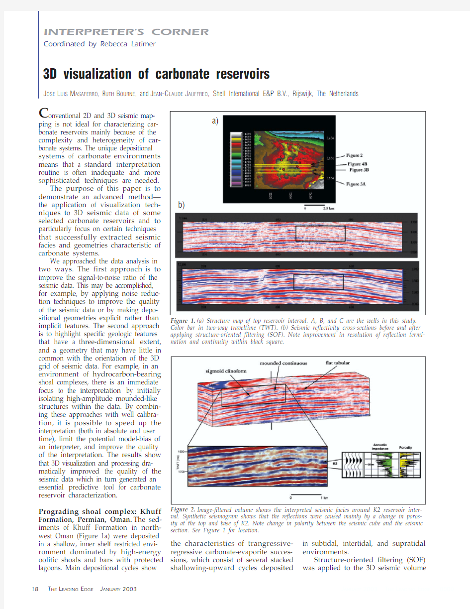
Prograding shoal complex: Khuff Formation, Permian, Oman.The sed-iments of Khuff Formation in north-west Oman (Figure 1a) were deposited in a shallow, inner shelf restricted envi-ronment dominated by high-energy oolitic shoals and bars with protected lagoons. Main depositional cycles show

the characteristics of trangressive-regressive carbonate-evaporite succes-sions, which consist of several stacked shallowing-upward cycles deposited in subtidal, intertidal, and supratidal environments.

Structure-oriented filtering (SOF)was applied to the 3D seismic volume

3D visualization of carbonate reservoirs

J OSE L UIS M ASAFERRO , R UTH B OURNE , and J EAN -C LAUDE J AUFFRED , Shell International E&P B.V., Rijswijk, The Netherlands

INTERPRETER’S CORNER

Coordinated by Rebecca Latimer

Figure 1.(a) Structure map of top reservoir interval. A, B, and C are the wells in this study.Color bar in two-way traveltime (TWT). (b) Seismic reflectivity cross-sections before and after applying structure-oriented filtering (SOF). Note improvement in resolution of reflection termi-nation and continuity within black square.

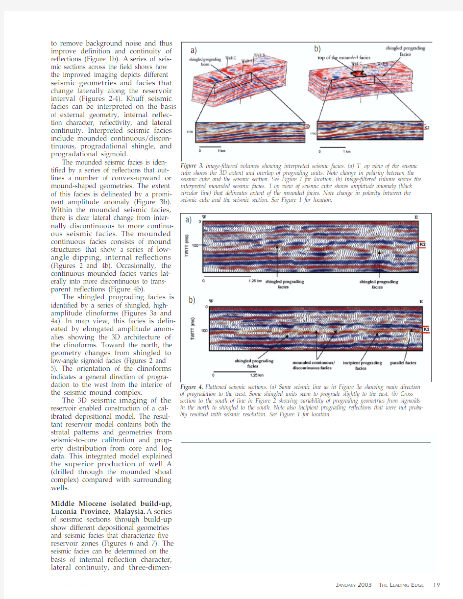
Figure 2.

Image-filtered volume shows the interpreted seismic facies around K2 reservoir inter-val. Synthetic seismogram shows that the reflections were caused mainly by a change in poros-ity at the top and base of K2. Note change in polarity between the seismic cube and the seismic section. See Figure 1 for location.

to remove background noise and thus improve definition and continuity of reflections (Figure 1b). A series of seis-mic sections across the field shows how the improved imaging depicts different seismic geometries and facies that change laterally along the reservoir interval (Figures 2-4). Khuff seismic facies can be interpreted on the basis of external geometry, internal reflec-tion character, reflectivity, and lateral continuity. Interpreted seismic facies include mounded continuous/discon-tinuous, progradational shingle, and progradational sigmoid.

The mounded seismic facies is iden-tified by a series of reflections that out-lines a number of convex-upward or mound-shaped geometries. The extent of this facies is delineated by a promi-nent amplitude anomaly (Figure 3b). Within the mounded seismic facies, there is clear lateral change from inter-nally discontinuous to more continu-ous seismic facies. The mounded continuous facies consists of mound structures that show a series of low-angle dipping, internal reflections (Figures 2 and 4b). Occasionally, the continuous mounded facies varies lat-erally into more discontinuous to trans-parent reflections (Figure 4b).

The shingled prograding facies is identified by a series of shingled, high-amplitude clinoforms (Figures 3a and 4a). In map view, this facies is delin-eated by elongated amplitude anom-alies showing the 3D architecture of the clinoforms. Toward the north, the geometry changes from shingled to low-angle sigmoid facies (Figures 2 and 5). The orientation of the clinoforms indicates a general direction of progra-dation to the west from the interior of the seismic mound complex.

The 3D seismic imaging of the reservoir enabled construction of a cal-ibrated depositional model. The resul-tant reservoir model contains both the stratal patterns and geometries from seismic-to-core calibration and prop-erty distribution from core and log data. This integrated model explained the superior production of well A (drilled through the mounded shoal complex) compared with surrounding wells.

Middle Miocene isolated build-up, Luconia Province, Malaysia.A series of seismic sections through build-up show different depositional geometries and seismic facies that characterize five reservoir zones (Figures 6 and 7). The seismic facies can be determined on the basis of internal reflection character, lateral continuity, and three-dimen-Figure 3.Image-filtered volumes showing interpreted seismic facies. (a) T op view of the seismic cube shows the 3D extent and overlap of prograding units. Note change in polarity between the seismic cube and the seismic section. See Figure 1 for location. (b) Image-filtered volume shows the interpreted mounded seismic facies. T op view of seismic cube shows amplitude anomaly (black circular line) that delineates extent of the mounded facies. Note change in polarity between the seismic cube and the seismic section. See Figure 1 for location.

Figure 4.Flattened seismic sections. (a) Same seismic line as in Figure 3a showing main direction of progradation to the west. Some shingled units seem to prograde slightly to the east. (b) Cross-section to the south of line in Figure 2 showing variability of prograding geometries from sigmoids in the north to shingled to the south. Note also incipient prograding reflections that were not proba-

bly resolved with seismic resolution. See Figure 1 for location.

sional geometry. Seismic facies were then calibrated using logs and part of one cored well.

The internal architecture of the build-up was previously interpreted,based on porosity contrast, to consist of five reservoir zones. Reservoir zones 1 and 2 exhibit a pronounced asym-metry in terms of seismic geometries (Figure 7). Zone 1, toward the west/southwest end of the platform, is char-acterized by high-amplitude, stacked-reef/mounded seismic facies (Figures 8 and 9). The remainder (approximately two-thirds) of the platform consists of

parallel, onlapping seismic reflections.Zone 2 shows N/NE-prograding seis-mic facies, which changes to more con-tinuous to transparent reflections (Figure 7). Seismic facies in zones 3 and 5 consist of high-amplitude, more or less continuous, flat-lying reflections (Figure 7). The intermediate reflection (marker reflection in Figure 6) is con-tinuous throughout the area and was used to flatten the seismic sections.Seismic facies in zone 4 is characterized by shingled seismic geometries in the southern part of the build-up changing to more continuous, high-amplitude

reflections toward the north. Zone 5shows more continuous reflections sometimes interrupted by localized mounded facies (Figure 7b).

Seismic images of the seismic reef/back-reef facies were extracted using gate-amplitude extractions, flat-tened semblance volumes and body-checking (Figures 8-10). Root mean square (rms) amplitude extraction using an amplitude window of 30 ms was applied to extract the reef/mounded seismic facies in zone 1 (Figure 8). The rms amplitude is calculated within a defined window (Figure 8b). Because of the extra reflections in the reef seismic facies, a constant amplitude window (30ms) was run through the entire seismic volume to give higher output amplitude values (red and green in Figure 8). The result is an amplitude map that shows a narrow distribution of higher ampli-tudes that correspond to the reef seismic facies confined to the W/SW part of the build-up. The back-reef/lagoonal seis-mic facies is also captured by the ampli-tude extraction as an amplitude anomaly adjacent to the reef seismic facies (Figure 8).

Coherence or semblance was also calculated from the reflectivity data and then flattened to the continuous reflec-tion interpreted as a flooding surface (Figure 9). A time slice through a flat-tened semblance volume shows a better-defined, linear seismic reef trend with high output values; lower semblance values represent the onlapping reflec-tions of the back-reef seismic facies more randomly distributed. The lowest sem-blance values (white in Figure 9) indicate greater similarities between traces that correspond to the more continuous seis-mic facies in the off-reef, lagoonal setting.Bodychecking was applied to the reflec-tivity volume to extract the high-ampli-tude seismic bodies of the seismic reef/back reef facies, by defining the maximum amplitude range of con-nected voxels for this particular seismic facies (Figure 10). The result is a 3D dis-tribution of detected bodies that shows the seismic reef tract and onlapping back-reef facies.

Upper Cretaceous ramp-type carbon-ate reservoir, Natih E Formation,Oman.SOF was applied to the origi-nal 3D seismic data for the study field to (Figures 11-12):

?reduce/suppress noise, improving lateral reflection continuity and seis-mic facies especially at the crest top (main reservoir area),

? improve reflection termination and geometries to better define reservoir

Figure 5.

Flattened seismic section and time slice of line in Figure 2 showing map extent of progra-dational sigmoids versus mounded seismic facies. Time slice was taken at the reservoir level indi-cated by the yellow line (108 ms flattened two-way traveltime).

Middle Miocene build-up. (b) Seismic section across the two wells with superimposed gamma ray logs. Black arrows are interpreted downlap reflections. (c) Gamma ray, density, and synthetic seis-mogram showing the five reservoir zones.

architecture,

?improve the definition of the top Natih E horizon by “smoothing out”previous noisy horizon interpreta-tion,

? produce attribute volumes such as semblance (Figure 13a), filtered sem-blance and combine dip and azimuth (Figure 13b) to constrain struc-tural/stratigraphic interpretation.

The original 3D data were used as a reference to compare and constrain the image-processed seismic. Three main seismic facies were recognized based on reflection geometry, reflec-tion continuity, and seismic reflectivity:

1) Prograding facies are restricted to the northern part of the field (Figure 11) and consist of low-angle dipping, high-amplitude reflections. The high ampli-tude character of the sigmoids is interrupted locally by dimming ampli-

tudes caused by the overlap between the termination of one sigmoid and the beginning of the next one. Time slices through the flattened reflectivity vol-ume show remarkably well the sig-moid overlapping and thus the east-west trend of the prograding units (Figure 14a). The calculated combined dip and azimuth volume (flattened on Natih E horizon) also shows the trend of progradation (Figure 13b).

2) Continuous/semicontinuous facies form the majority of seismic facies observed within the Natih E interval (Figure 11b). It is characterized by high-amplitude, parallel to subparallel seis-mic reflections. Occasionally, reflection continuity is disrupted, either by faults or by remnant seismic noise

3) The chaotic-to-transparent facies is represented by discontinuous reflec-tions with low-to-moderate reflectivity. This facies is associated with internal faulting and/or nonorganized noise and occurs at the southern crestal part of the field (Figure 11b). Possible gas-escape effects also obscure reflection definition in the crestal part of the field. The areal distribution of this facies is shown clearly in the flattened reflec-tivity volume at different levels within the reservoir (Figure 11).

Analysis of seismic facies and geometries provided an initial frame-work to constrain the lateral strati-graphic correlation based on core and log data. Permeable units within aggra-dational geometries in the crestal area (interpreted as ramp-crest shoal com-plex) seem to continue into the water leg (Figure 11b). This interpretation evolved into a subsurface model sce-nario that could explain the provenance of high water cuts observed in the field.Figure 7.Prograding reef system initiated as smaller build-ups that then coalesced through time filling in the space available to form a larger platform. (a) Flattened seismic section showing charac-teristic seismic facies and lateral heterogeneity within the five reservoir zones. (b) Seismic section showing seismic reef facies and prograding foresets within reservoir zone 5.

Figure 8.(a) Gate amplitude map showing map distribution of the interpreted seismic reef facies. Red/green = high amplitudes and blue/light blue = low amplitude. (b) Flattened seismic section

showing the reef/back reef seismic facies. Amplitude gate of 30 ms indicated with red arrows.

Malampaya Field, Philippines.Texture mapping was applied to a seg-mented seismic volume defined by the two horizons corresponding to the top and base of the reservoir in Malampaya Field. Two distinctive interpreted seis-mic facies were identified and then run

as training sets through the seismic vol-ume (Figure 15a). The first training set represents the seismic character simi-lar to the western part of the build-up (chaotic, steeply dipping discontinu-ous reflections). The second represents seismic facies from the interior of the

Figure 9.Flattened volume semblance showing high semblance values (dark blue) that correspond to the reef seismic facies. Intermediate semblance values represent the less linear back-reef deposits.Low semblance values indicate flat-lying reflections interpreted as lagoonal seismic facies. Red arrows indicate interpreted paleo-wind directions for the Middle Miocene.

Figure 10.(a) Example of bodychecking defined for amplitude range of 0-60. The result shows the extracted bodies contained within that range. (b) Bodychecking on reflectivity volume using cali-brated amplitude ranges to extract reef/back-reef seismic bodies. Red, blue, and pink extracted bodies show the linear space distribution of the seismic reef tract. Green and orange extracted bodies repre-

sent the seismic back-reef deposits.

build-up (high-amplitude, continuous,flat-lying reflections). Several attributes related to amplitude, continuity and similarity between traces, and dip and azimuth were calculated to extract these seismic facies. The results are shown in Figure 15a, which represent slices through the calculated texture volume. Blue represents the calculated texture for the marginal reef-related seismic facies and light green the more internal seismic lagoonal facies. The two seismic textures were exported to the static reservoir simulator and used to constrain different model scenarios.

Bodychecking was carried out on the porosity volume generated from the acoustic impedance data within the reservoir unit. The objective was to ana-lyze the porosity distribution and investigate sizeable porosity bodies that could be used to constrain the reservoir modeling. Bodychecking was applied over a wide range of “poros-ity” thresholds, and porosity bodies with 2% threshold were extracted.Figure 15b shows the connected bod-ies displayed in the same volume with different colors, making it possible to analyze the distribution of the con-nected porosities and the relationship between porosity ranges. The porosity distribution shows more seismic-derived porosities in the northern part of the Malampaya build-up than in the south.

https://www.360docs.net/doc/a06929448.html,bining 3D seismic visualization techniques with core and log calibration provided a robust methodology for interpretation of car-bonate reservoirs. Case studies in this paper demonstrate the use of the dif-ferent image processing techniques to highlight key seismic geometries and facies for various types of carbonate

Figure 11.(a) Isochore map of the Natih E interval and seismic facies map. (b) Interpreted seismic section across the field. OWC = oil water contact.

Figure 12.Seismic reflectivity cross-section before and after applying structure-oriented filtering.

Y ellow arrows indicate significant improvement in continuity and definition at reflection termina-tions. T runcation and progradation geometries are now more obvious in the filtered volume. Red dots are artifacts from image filtering.

systems. These studies showed that accurate seismic imaging of the reser-voir architecture becomes an impor-tant predictive tool for reservoir characterization because it helped to build a 3D geologic framework within which depositional facies can be dis-tributed in time and space. Calculation of volume-based attributes produced new volumes of data that helped extract the 3D geometries within the reservoir.

In the Permian Khuff example,reservoir image-filtering considerably improved reflection termination and subsequent delineation of the topo-graphically distinct shoal grainstone complex from the prograding units.Integration of seismic geometries and facies with core and log data provided a reliable geologic and static model that could explain well performance.

In the Middle Miocene Luconian isolated build-up, a combination of vol-ume semblance, gate-amplitude extrac-tions, and bodychecking techniques allowed identification of depositional geometries within the five reservoir zones. Extracted geometries showed the 3D spatial distribution of the seis-mic facies through time. Transgressive portions of the cycles are expressed as flat-lying, high-amplitude reflections.Highstand conditions provided more accommodation space in which aggrading reef/back-reef and pro-grading seismic facies developed.Recognition of seismic facies hetero-geneities had implications on the final building of the static model in terms of lateral correlation of stratigraphic units between the wells and on the 3D dis-tribution of petrophysical properties.

Application of SOF dramatically improved definition and continuity of reflections in Natih E reservoir. Time slices through flattened, image-filtered reflectivity, semblance, and combined volume dip and azimuth helped delin-eate the reservoir zone. Integration of seismic interpretation calibrated with the cored well, logs, and outcrop analogs produced a static reservoir model that could explain high water cuts in the field. Texture and body-checking were successfully applied to the Malampaya seismic data set to quickly identify and classify seismic facies and to extract the seismically detected good porous zones within the reservoir. The results showed the vol-ume distribution of seismic facies and porosity zones, which were used as input to target potential good wells and as a reference to constrain reservoir quality distribution.

Figure 13.(a) Semblance volume calculated from the original reflectivity data and from the image filtered data. Red square indicates approximate location of the field. (b) Combined dip and azimuth time slices applied to flattened reflectivity data showing orientation of prograding geometries. At 0time no preferred orientation is observed. Orientation of clinoforms is obvious at 16 ms below the flattened reference horizon.

Figure 14.(a) Time slices through flattened, filtered reflectivity volume. Time slices at 16 and 20ms below the flattened reference horizon (top Natih E) show amplitude dimming caused by the overlapping between termination of one clinoform and beginning of the next (red arrows). (b)

Flattened seismic section showing low-angle progradation. Flatten horizon = top Natih E. Red dots are artifacts from image filtering process.

Suggested reading.“The coherence cube” by Bahorich and Farmer (TLE, 1995). “Integrated 3D reservoir model-ing based on 3D seismic: The Tertiary Malampaya and Camago build-ups, off-shore Palawan, Philippines” by Grotsch and Mercadier (AAPG Bulletin, 1999).“Fast structural interpretation with struc-ture-oriented filtering” by H?cker and Fehmers (TLE, 2002).T L E Acknowledgments: This paper is a modified ver-sion of a more extended paper which will be pub-lished in an upcoming AAPG special volume. The authors thank Shell International Exploration and Production B.V. for permission to publish this paper. Petronas, Sarawak Shell Berhad, Shell Philippines, and Petroleum Development Oman are gratefully acknowledged for giving permission to publish the data in the paper. We acknowledge the contribution of the Seismic Volume Interpretation Team (VOICE) and the Carbonate Development Team within Shell Technology Applications and Research (SEPTAR). Our paper has benefited from numerous discussions with Gregor Eberli, Updesh Singh, Volker Vahrenkamp, and Taury Smith.

Corresponding author: JoseLuis.Massaferro@ https://www.360docs.net/doc/a06929448.html, b)

Figure 15.(a) T exture classification applied to prestack depth-migrated

(PSDM) data. The texture analysis was based on second moment, semblance,

and co-occurency. Green = continuous, high-amplitude reflections corre-

sponding to the intra-buildup, lagoonal seismic facies. Blue = chaotic, steeply

dipping, discontinuous, marginal seismic facies. (b) Bodychecking results for

calculated porosity from acoustic impedance data. Cross-section and time

slices show porosity distribution.