Peculiar velocity effects in high-resolution microwave background experiments

a r X i v :a s t r o -p h /0112457v 1 19 D e c 2001Peculiar velocity e?ects in high-resolution microwave background experiments

Anthony Challinor 1,?and Floor van Leeuwen 2,?

1Astrophysics Group,Cavendish Laboratory,Madingley Road,Cambridge CB3OHE,UK.2Institute of Astronomy,Madingley Road,Cambridge,CB30HA,UK.

We investigate the impact of peculiar velocity e?ects due to the motion of the solar system relative to the microwave background (CMB)on high resolution CMB experiments.It is well known that on the largest angular scales the combined e?ects of Doppler shifts and aberration are important;the lowest Legendre multipoles of total intensity receive power from the large CMB monopole in transforming from the CMB frame.On small angular scales aberration dominates and is shown here to lead to signi?cant distortions of the total intensity and polarization multipoles in transforming from the rest frame of the CMB to the frame of the solar system.We provide convenient analytic results for the distortions as series expansions in the relative velocity of the two frames,but at the highest resolutions a numerical quadrature is required.Although many of the high resolution multipoles themselves are severely distorted by the frame transformations,we show that their statistical properties distort by only an insigni?cant amount.Therefore,cosmological parameter estimation is insensitive to the transformation from the CMB frame (where theoretical predictions are calculated)to the rest frame of the experiment.I.INTRODUCTION The impressive advances being made in sensitivity and resolution of microwave background (CMB)experiments demand that careful attention be paid to potential systematic e?ects in the analysis pipeline.Such e?ects can arise from imperfect modelling of the instrument,e.g.approximations in modelling the beam [1,2,3,4],or incomplete knowledge of the pointing,but also from more fundamental e?ects such as inaccurate separation of foregrounds (see e.g.Refs.[5,6]for reviews).In this paper we consider errors that may arise due to neglect of the peculiar motion of the experiment relative to the CMB rest frame (that frame in which the CMB dipole vanishes).For short duration experiments (e.g.balloon ?ights such as MAXIMA [7]and BOOMERANG [8])the relative velocity is constant over the timescale of the experiment,but for experiments conducted over a few months or longer,and particularly for satellite surveys [9,10,11],the variation in the relative velocity adds additional complications.In principle,the modulation of the aberration arising from any variation in the relative velocity must be accounted for with a more re?ned pointing model for the experiment [12,13]when making a map.For a relative speed of βc (where c is the speed of light and β～1.23×10?3for the solar-system barycenter relative to the CMB frame),the r.m.s.photon Doppler shifts and de?ection angles are β/√2/3βrespectively.Despite these small values,signi?cant distortions of the spherical multipoles of the total intensity and polarization ?elds do arise.A well known example is provided by the CMB dipole seen on earth,which,given the observed spectrum,arises from the transformation of the monopole in the CMB frame.More generally,on the largest angular scales

the combined e?ects of Doppler shifts and aberration couple the total intensity monopole and dipole into the l th multipoles at the level O (βl )and O (βl ?1)respectively.Given the size of the non-cosmological monopole,annual modulation of the dipole by the variation in the relative velocity of the earth in the CMB frame must be considered in long duration experiments.

In this paper we concentrate on the e?ects of peculiar velocities on small angular scale features in the microwave sky.On such scales,aberration dominates the distortions and becomes particularly acute when the angular scales of interest,O (1/l ),drop below the r.m.s.de?ection angle,i.e.l >～800for the transformation from the CMB frame to that of the solar system.We provide simple analytic results for these distortions to the total intensity and polarization ?elds as power series in the relative velocity β.The power series converge rather slowly at the highest multipoles for most values of the azimuthal index m [the leading-order corrections go like O (lβ)]but the distortions can still easily be found semi-analytically with a one-dimensional quadrature.If the transformations of the multipoles carried through to their statistical properties,theoretical power spectra computed in linear theory (e.g.with standard Boltzmann

codes [14,15])would not accurately

describe the statistics of the high resolution multipoles observed on earth.(The theoretical power spectra would still be accurate in the CMB frame.)It is straightforward to calculate the statistical correlations of the multipoles observed on earth.Fortunately,as we show here,the statistical corrections due to peculiar velocity e?ects turn out to be negligible despite the large corrections to the individual multipoles.It follows that for the purposes of high resolution power spectrum and parameter estimation,the transformation from the CMB frame can be neglected.

This paper is arranged as follows.In Sec.II we describe the transformation laws for the total intensity multipoles in speci?c intensity and frequency-integrated forms.Convenient series expansions in βof the transformations are provided,and their properties under rotations of the reference frames are described.The statistical poperties of the transformed multipoles are investigated by constructing rotationally-invariant power spectrum estimators and full correlation matrices.In Sec.III we discuss the geometry of the frame transformations for linear polarization,and present power series expansions for the transformations of the multipoles.The behaviour under rotations and parity are also outlined.Power spectra estimators and correlation matrices are constructed,and cross correlations with the total intensity are considered.Some implications of our results for survey missions are discussed in Sec.IV,which is followed by our conclusions in Sec.V.An appendix provides details of the evaluation of the multipole transformations as power series in β.

We use units with c =1.

II.TRANSFORMATION LA WS FOR TOTAL INTENSITY

We consider the microwave sky as seen by two observers at the same event.Observer S is equipped with a comoving tetrad {(e μ)a },μ={0,1,2,3},and observer S ′carries the Lorentz-boosted tetrad {(e ′μ)a }.The relative velocity of S ′as seen by S has components on {(e i )a },i ={1,2,3},which we denote by the spatial vector v ,which has magnitude β.The S observer receives a photon with four-momentum p a when their line of sight is along ?n ,so the photon propagation direction is ??n

.For S the photon frequency is νwhere hν=p a (e 0)a (h is Planck’s constant),while S ′observes frequency

ν′=νγ(1+?n

·v ),(1)where γ?2=1?β2.The line of sight in S ′is ?n ′= ?n ·?v +βγ(1+?n ·v ),(2)

where ?v

is a unit vector in the direction of the relative velocity.Denoting the sky brightness in total intensity seen by S as I (ν,?n

),the brightness seen by S ′is (e.g.Ref.[16])I ′(ν′,?n

′)=I (ν,?n ) ν′ν 4.(5)

Expanding I (?n )in spherical harmonics,we ?nd the multipole transformation law a I ′lm = l ′m ′

a I l ′m ′

d?n [γ(1+?n ·v )]2Y l ′m ′(?n )Y ?lm (?n ′),=

l ′m ′K (lm )(lm )′a I l ′m ′(6)

where a I lm= dνa I lm(ν).The second equality de?nes the kernel K(lm)(lm)′which relates the frequency-integrated multipoles in S and S′.Dividing a I lm by four times the average?ux per solid angle gives the multipoles of the gauge-invariant temperature anisotropy in linear theory(e.g.Refs.[17,18]).

If we choose the spacelike vectors of the tetrad{(eμ)a}so that the relative velocity is along(e3)a,the multipole transformation law becomes block-diagonal,K(lm)(lm)′∝δmm′,with no coupling between di?erent m modes.The kernel for a general con?guration can then be inferred from its transformation properties under rotations described in Sec.II A.In the appendix we evaluate Eq.(4)as a series expansion inβfor general spin-weight functions,including terms up to O(β2),for the case where v is aligned with(e3)a.The expression is cumbersome,partly due to the fact that the transformation law is non-local in frequency.For large l the aberration e?ect dominates Doppler shifts and the frequency spectrum of the multipoles is preserved by the transformation.We also give the result obtained by integrating over frequency;setting s=0in Eq.(A7)we?nd the series expansion of the kernel K(lm)(lm)′up to O(β2):

K(lm)(l′m)=δll′ 1+1

2(l+2)(l+3)+δl(l′?2)β2C(l+2)m C(l+1)m

1 (l2?m2)(l2?s2)

l).For lβ?1,the departures of the kernel from the identityδll′δmm′are very small,giving negligible distortions to the multipoles except for l close to unity when the non-zero coupling to the(large)monopole can give signi?cant distortions,as described in Sec.I.

A.Rotational properties

If we rotate the relative velocity v to D v1keeping the tetrad(eμ)a?xed,[thus inducing a transformation of the Lorentz-boosted tetrad(e′μ)a],the frequency-integrated multipoles continue to be given by Eq.(6),but with v replaced by D v in?n′[Eq.(2)]and in(1+?n·v).With the change of integration variable?n→D?n,the integral de?ning the transformed kernel K(lm)(lm)′(D v)becomes

d?nγ2(1+?n·v)Y l′m′(D?n)Y?lm(D?n′)= d?nγ2(1+?n·v)D?1Y l′m′(?n)[D?1Y lm(?n′)]?,(9)

where D?1Y l′m′(?n)= m′′D l?m′m′′Y lm′′(?n)with D l mm′a Wigner D-matrix.(Our conventions for D-matrices follow Refs.[19,20].)It follows that the transformed kernel is given by

K(lm)(lm)′(D v)= MM′D l mM K(lM)(lM)′(v)D l′?m′M′.(10)

Instead of rotating the(physical)relative velocity of S and S′,we could imagine rotating the spatial triad(e i)a→D(e i)a.Under this coordinate transformation,the Lorentz-boosted frame vectors transform similarly:(e′i)a→D(e′i)a.

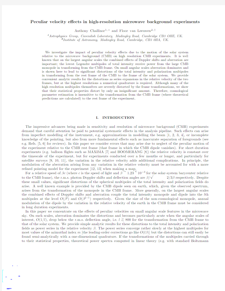
FIG.1:Representative elements of the frequency-integrated kernel K(lm)(lm)′evaluated with the relative velocity(β=1.23×10?3)along(e3)a.The results of a numerical integration of Eq.(6)are shown in dark gray,while results based on the series expansion(7)are shown in light gray.The smaller(absolute values)of the two are shown in the foreground.Elements are shown for l=1500(left),l=700(middle),and l=50(right),with m=0(top)and m=l(bottom).

For a?xed sky,the multipoles seen by S and S′transform according to e.g.a I lm→ m′D l?m′m a I lm′(which is equivalent to rotating the sky with D?1leaving the tetrad?xed).It follows that under coordinate rotations,the kernel transforms as

K(lm)(lm)′→D l?Mm K(lM)(lM)′D l′M′m′.(11) Note that the(passive)rotation of the frame vectors by D?1has the same e?ect on the kernel as the(active)rotation of the relative velocity v by D,as expected.

Finally,we consider(active)parity transformations v→?v with the tetrad(eμ)a held?https://www.360docs.net/doc/bd8555995.html,ing Y lm(??n)= (?1)l Y lm(?n)it is straightforward to show that

K(lm)(lm)′(?v)=(?1)l+l′K(lm)(lm)′(v).(12) The behaviour of the kernel under parity ensures that if we simultaneously invert v and the sky[a I lm→(?1)l a I lm], the multipoles seen by S′transform to(?1)l a I′lm.

These transformation properties of the kernel under rotations allow one to generalise Eq.(7)easily to the case where v is not aligned with(e3)a.

B.Power spectrum estimators

We have seen how aberration e?ects lead to signi?cant distortions of some of the high-l multipoles in transforming from the CMB frame to the frame of the experiment.In the next two subsections we investigate the impact of these distortions on the statistical properties of the multipoles.

We assume that in the CMB frame(S)the second-order statistics of the anisotropies are summarised by

a I lm a I?l′m′ =C II lδll′δmm′,(13)

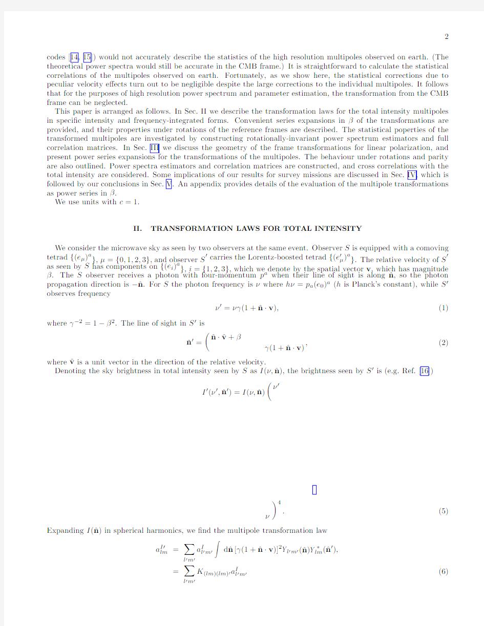
FIG.2:Representative elements of the kernel W ll′evaluated with relative velocityβ=1.23×10?3.The results of a numerical integration of are shown in dark gray,while results based on the series expansion(16)are shown in light gray.The smaller (absolute values)of the two are shown in the foreground.Elements are shown for l=1500(left),l=700(middle),and l=50 (right).

appropriate to a statistically-isotropic ensemble with power spectrum C II l.(The averaging is over an ensemble of CMB realizations.)It is this C l for l≥2that is computed with linear perturbation theory in standard Boltzmann codes(e.g.Refs.[14,15]).

We begin by considering the quadratic statistic

1

?C II′

l≡

2l+1 l′mm′|K(lm)(lm)′|2C II l′

≡ l′W ll′C II l′.(15)

The kernel W ll′depends only on the relative speedβand not the direction?v,so we can always evaluate it with v aligned with(e3)a.

The series expansion(7)of K(lm)(lm′)can be used to evaluate W ll′.Correct to O(β2)we?nd

W ll′=δll′ 1?13(2l+1)+δl(l′?1)β2(l?2)2(l+1)

using the integral expression(6)for K(lm)(lm)′.The result simpli?es to

l′W ll′=γ45β4 ,(18) on using the completeness relation

lm s Y lm(?n1)s Y?lm(?n2)=δ(?n1??n2),(19) and the addition theorem for the spherical harmonics.The series expansion of Eq.(18)agrees with Eq.(17).We

conclude that despite the fact that the multipoles themselves can be severely distorted by aberration for lβ>～1in passing from the CMB frame to that of the solar system,the quadratic power spectrum estimator is negligibly biased

since the e?ect of the velocity transformation is to convolve the power spectrum with a narrow kernel W ll′that sums to very nearly unity.

C.Signal covariance matrix

Assuming Gaussian statistics in the CMB frame,the multipoles a I′lm in S′will also be distributed according to a multivariate Gaussian since the transformation(6)is linear.In this case,the covariance matrix a I′lm a I′?l′m′ contains all statistical information about the anisotropies in S′,and as such is an essential element of optimal power spectrum estimation.

If we make use of Eq.(13),the covariance matrix in S′reduces to

a I′lm a I′?l′m′ = LM K(lm)(LM)K?(lm)′(LM)C II L.(20)

The presence of the preferred direction?v breaks statistical isotropy in S′,and the multipoles are correlated for l=l′and m=m′.The structure of the covariance matrix in S′depends on the choice of the spatial triad(e i)a with respect to the relative velocity of the two observers.Aligning(e3)a with v,the m-modes decouple in K(lm)(lm)′and so also in the covariance matrix.Furthermore,for the values ofβof interest here(β?1),the kernel K(lm)(lm)′falls rapidly to zero for l and l′di?ering by more than a few(see Fig.1),so the same will be true of the covariance matrix.It follows that we can approximate

a I′lm a I′?l′m′ ≈C II l LM K(lm)(LM)K?(lm)′(LM).(21)

(Pulling out C II l′instead will give essentially the same result for smooth power spectra.)The summation in Eq.(21) is most easily evaluated by substituting the integral representation(6)for K(lm)(LM)and using the completeness relation(19).We?nd that LM K(lm)(LM)K?(lm)′(LM)reduces to the integral

d?n[γ(1+?n·v)]4Y?lm(?n′)Y l′m′(?n′)= d?n′[γ(1??n′·v)]?6Y?lm(?n′)Y l′m′(?n′),(22)

where we changed the integration variable to?n′and usedγ(1+?n·v)=[γ(1??n′·v)]?1.Note that both spherical harmonics have the same argument in the integrand,so we don’t expect the same O(lβ)terms at high l that arise in the kernel K(lm)(lm)′.Eq.(22)can easily be evaluated for(e3)a along v(in which case there is no coupling between di?erent m)by expanding inβ:

LM K(lm)(LM)K?(l′m)(LM)=δll′[1+3β2(7C2(l+1)m+7C2lm?1)]+δl(l′+1)6βC lm+δl(l′?1)6βC(l+1)m

+δl(l′+2)21β2C lm C(l?1)m+δl(l′?2)21β2C(l+2)m C(l+1)m+O(β3).(23) This result for the covariance matrix in S′could easily be used in maximum-likelihood power spectrum estimation (see e.g.Ref.[21])to correct for the bias due to peculiar velocity e?ects.However,since the leading corrections are only O(β),even at high l,the e?ects will be negligible.

III.TRANSFORMATION LA WS FOR LINEAR POLARIZATION

The linearly polarized brightness in S is described by Stokes parameters Q (ν,?n

)and U (ν,?n ).The Stokes parameters depend on a speci?c choice of orthonormal basis vectors {m 1,m 2}for each line of sight ?n .If {m 1,m 2,??n }form a right-handed orthonormal set,the Stokes parameters are related to the linear polarization tensor by

P ab =1

ν 3,(25)

and similarly for U ,provided that the basis vectors are transformed according to

[22]m

′

i

=

m

i +(γ?1)m i ·?v ?v ?γm i ·v ?n ′,(26)

where i =1,2.It is straightforward to verify that this transformation law preserves orthonormality,and also that m ′i is obtained from m i by parallel transport on the unit sphere along the great circle through ?n

and ?n ′(and so through ?v

also).In terms of the polarization tensor,the frame transformation law can be written as P ′ab (ν′,?n ′)=P ab (ν,?n

;v ) ν′√

√

i √

2,so that Eq.(29)can be written as

(a E ′lm ±ia B ′lm )(ν′)= l ′m ′(a E l ′m ′±ia B l ′m ′)(ν)

d?n γ(1+?n ·v )±2Y l ′m ′(?n )±2Y ?lm (?n ′).(32)

2times the gradient (G )and curl (C )multipoles introduced in Refs.[23,24].With this convention the power

spectra of the electric and magnetic multipoles agree with those de?ned in the spin-weight formalism [25,26].

The integral on the right-hand side is evaluated as a power series inβfor general spin-weight s in the appendix. For our purposes it will be more convenient to consider the frequency-integrated multipoles,e.g.a E lm= dνa E lm(ν). Integrating Eq.(29)over frequency,we?nd

a E′lm= l′m′+K(lm)(lm)′a E l′m′+i?K(lm)(lm)′a B l′m′,(33)

a B′lm= l′m′+K(lm)(lm)′a B l′m′?i?K(lm)(lm)′a E l′m′,(34) where the kernels

+

K(lm)(lm)′= d?n[γ(1+?n·v)]2Y G ab (lm)′(?n;v)Y G?(lm)ab(?n′)= d?n[γ(1+?n·v)]2Y C ab (lm)′(?n;v)Y C?(lm)ab(?n′),(35)?

K(lm)(lm)′=?i d?n[γ(1+?n·v)]2Y C ab (lm)′(?n;v)Y G?(lm)ab(?n′)=i d?n[γ(1+?n·v)]2Y G ab (lm)′(?n;v)Y C?(lm)ab(?n′).(36)

The behaviour of±K(lm)(lm)′under rotations v→D v is the same as for the total intensity kernel,Eq.(10),since the tensor harmonics transform under rigid rotations with the same D-matrices as the scalar harmonics[1].This property of the tensor harmonics also ensures that under rotations of the coordinate system,(e i)a→D(e i)a,the electric and magnetic multipoles transform irreducibly to e.g. m′D l?m′m a E lm′.Under inversion of v with(eμ)a held ?xed,the kernels transform to

+

K(lm)(lm)′(?v)=(?1)l+l′+K(lm)(lm)′(v),(37)

?

K(lm)(lm)′(?v)=?(?1)l+l′?K(lm)(lm)′(v),(38) so that under simultaneous inversion of the sky in S,a E lm→(?1)l a E lm and a B lm→(?1)l+1a B lm,and inversion of v,the multipoles in S′transform like those in S.

The frequency-integrated kernels are most simply evaluated with v along(e3)a.In this case the m-modes decouple, as with the total intensity.Writing±K=(2K±?2K)/2,we can use Eq.(A7),which evaluates s K(lm)(lm)′as a series correct to O(β2),to show that

+

K(lm)(l′m)=δll′ 1+1l(l+1)+24m2

2(l+2)(l+3)+δl(l′?2)β22C(l+2)m2C(l+1)m

1

l(l+1)?δl(l′+1)2C lm(l+3)6β2m

l(l+2)

.(40)

(Equivalent results,correct to O(β),have already been worked out in1+3covariant form[22].)The kernel?K(lm)(lm)′is suppressed at high l.It receives comparable contributions from Doppler and aberration e?ects for all l[see Eq.(A6)]

in contrast to the+K(lm)(lm)′and the total intensity kernel K(lm)(lm)′which are dominated by aberration e?ects at high l.The series expansion of+K(lm)(lm)′is slow to converge for lβ>～1when|m|?l,and there are large distortions to the electric and magnetic multipoles for these indices.Electric multipoles nearby in l couple in strongly to distort

a E lm,and similarly for the magnetic multipoles.For l?1the kernel+K(lm)(lm)′is almost indistinguishable from the total intensity kernel K(lm)(lm)′.The cross contamination of e.g.B by E due to the frame transformation is much weaker,with the maximal e?ect～O(β/l)at leading order occuring for|m|≈l.[Note that,as with+K(lm)(lm)′,the convergence of of Eq.(40)is slow for lβ>～1when|m|?l.]The transfer of power from E to B is potentially the most interesting e?ect since in the absence of astrophysical foregrounds,in?ationary models predict that magnetic polarization in the CMB frame on scales larger than a degree or so arises only from gravitational waves.However,on these scales a gravity wave background comprising only one percent of the large-angle temperature anisotropy would have B power far in excess of that generated in the frame of the experiment by transforming E from the CMB frame. On sub-degrees scales,where any primordial B-polarization is expected to be very small,other non-linear e?ects, most notably weak lensing of E[28],will dominate the B signal produced by the velocity transformation.

A.Power spectrum estimators

The second-order statistics of the polarization multipoles in the CMB frame,assuming statistical isotropy and parity invariance,de?ne power spectra:

a E lm a E?l′m′ =δll′δmm′C EE l,(41)

a B lm a B?l′m′ =δll′δmm′C BB l,(42)

a E lm a I?l′m′ =δll′δmm′C IE l,(43) with no correlations between B and E or I.We can form estimators of these power spectra from the multipoles in S′by analogy with Eq.(14),e.g.

?C IE′l =

1

2l+1 l′m′m|+K(lm)(lm)′|2C EE l′+|?K(lm)(lm)′|2C BB l′,(45) ?C BB′l =1

2l+1 l′m′m+K(lm)(lm)′K?(lm)(lm)′C IE l′.(47) Substituting the power series expressions for the kernels and performing the summations over m and m′we?nd 1

3

β2(l+4)(l?3) +δl(l′+1)β2(l+3)2(l2?4)

3(l+1)(2l+1)

,(48) 1

l(l+1)

,(49) and

1

3

β2(l2+l?10) +δl(l′+1)β2 3(2l+1)

+δl(l′?1)β2 3(2l+1),(50)

correct to O(β2).For l?1the right-hand sides of Eqs.(48)and(50)are almost equal to each other and to the kernel W ll′which determines the bias in the total-intensity estimator?C II′l.As with the total intensity,the series in Eqs.(48–50)are slow to converge for lβ>～1.The bias of?C BB′l by E-polarization is controlled by mm′|?K(lm)(lm)′|2/(2l+1),

which falls o?rapidly with l.In Fig.3we compare this contribution to the expected ?C BB′

l with the B-polarization power spectrum due to primordial gravity waves and weak lensing of the E-polarization.The cosmological model is a Lambda,cold dark matter(ΛCDM)in which gravity waves contribute one percent to the large-angle temperature anisotropy.As remarked earlier,the contamination arising from the frame transformation is well below the expected C BB

l

in such a model.

The means of the estimators?C EB′

l and?C EB′

l

,de?ned by analogy with?C IE′

l

,would vanish in the absence of peculiar

velocity e?ects(and foregrounds)due to parity.The velocity transformations preserve these zero means since

mm′+K(lm)(lm)′?K?(lm)(lm)′= mm′?K(lm)(lm)′K?(lm)(lm)′=0.(51)

FIG.3:Contribution of C EE

l to the mean estimator ?C BB′

l in aΛCDM model with one percent contribution to the total-

intensity quadrupole from gravity waves.This velocity e?ect is compared with C BB

l(in the CMB frame)due to primordial gravity waves(solid line)and weak lensing of the E-polarization(dashed line).

These results are easily proved by choosing v along(e3)a so that all kernels are real,and using the general results

±K?

(lm)(lm)′

=±(?1)m+m′±K(l?m)(l′?m′)and K?

(lm)(lm)′

=(?1)m+m′K(l?m)(l′?m′).

The kernels represented by the left-hand sides of Eqs.(48)–(50)fall o?su?ciently rapidly with|l′?l|that they are

narrow compared to expected features in the primordial power spectra3.Following the analysis in Sec.II B we can

pull out C EE

l′,C BB

l′

,and C IE l′at l′=l from the summations in Eqs.(45)–(47).Performing the sums over l′,we?nd 1

l(l+1)

,(52) 1

l(l+1)

,(53)

1

3

β2 2l+1+ 2l+1?l2?l+10 ,(54)

correct to O(β2).For large l the right-hand sides of Eqs.(52)and(54)approach1+4β2;as with the total intensity, there is a negligible scaling of the amplitude of the power spectra estimated in the S′frame due to the frame transformation.Note that

1

2(2l+1) mm′l′[|2K(lm)(lm)′|2+|?2K(lm)(lm)′|2]

=γ4 1+2β2+1

3At low l the polarization power spectra vary rapidly(as power laws)with l.Over this part of the spectrum the approximation that the power is approximately constant over the width of the convolving kernel is still valid since the latter are essentially Kronecker deltas at low l.

B.Signal covariance matrices

The calculation of the covariance matrix of the polarization multipoles in S′follows that for the total intensity given in Sec.II C.For smooth power spectra we can approximate

a E′lm a E′?l′m′ ≈C EE l LM+K(lm)(LM)+K?(lm)′(LM)+C BB l LM?K(lm)(LM)?K?(lm)′(LM),(56)

a B′lm a B′?l′m′ ≈C BB l LM+K(lm)(LM)+K?(lm)′(LM)+C EE l LM?K(lm)(LM)?K?(lm)′(LM),(57)

a E′lm a I′?l′m′ ≈C IE l LM+K(lm)(LM)K?(lm)′(LM).(58) The remaining correlators would vanish for v=0due to parity invariance.For non-zero v we can approximate

a E′lm a B′?l′m′ ≈iC EE l LM+K(lm)(LM)?K?(lm)′(LM)+iC BB l LM?K(lm)(LM)+K?(lm)′(LM),(59)

a B′lm a I′?l′m′ ≈?iC IE l LM?K(lm)(LM)K?(lm)′(LM).(60)

If we align v with(e3)a we can evaluate these expressions by substituting for the series expansions of the kernels from Eqs.(39)and(40).The m modes decouple and we?nd

LM+K(lm)(LM)+K?(l′m)(LM)=δll′ 1+3β2 72C2(l+1)m+72C2lm+16m2

l2(l+1)2

,(62) and

LM+K(lm)(LM)K?(l′m)(LM)=δll′ 1+1

2

δl(l′+2)β2[(l+2)(l+3)2C lm2C(l?1)m+(l?3)(l?4)C lm C(l?1)m

?2(l+3)(l?4)2C(l?1)m C lm]+1

2?155+84m2

l?

3(7+4m2)

l?29+12m2

4?

5

16l2

+δl(l′?2)β2 212l?223+84m2

It is worth noting that

LM(+K(lm)(LM)+K?(l′m)(LM)+?K(lm)(LM)?K?(l′m)(LM))

=

1

l(l+1)?δl(l′+1)2C lm(7l+3)

6β2m

l(l+1)(l+2)

,(66) LM?K(lm)(LM)K?(l′m)(LM)=?δll′6βm l(l+1)(l?1)

+δl(l′?1)[(l+1)(l?2)2C(l+1)m?(l+4)(l+2)C(l+1)m]6β2m

2 d?n[γ(1??n·v)]?6[2Y?lm(?n)2Y l′m(?n)??2Y?lm(?n)?2Y l′m(?n)].(69)

This result is easily shown to be consistent with Eqs.(66)and(68).

IV.IMPLICATIONS FOR SUR VEY MISSIONS

For experiments which observe for less than a month or so the velocity of the instrument relative to the CMB frame can reasonably be considered constant.In this case a map in the frame of the instrument can be made with no account of the e?ects considered in this paper.Accounting for the peculiar velocity relative to the CMB frame can be deferred until the statistical properties of the map are considered.As we have shown here,peculiar velocity e?ects can safely be ignored when estimating smooth power spectra since the estimated power spectra are essentially convolutions of the spectra in the CMB frame(which we can reliably compute with linear perturbation theory)with narrow kernels that integrates to unity.

For survey experiments that observe for the order of a year or more the variation in the orbital velocity of the instrument adds another potential complication.Modulation of the dipole by the orbital velocity of the earth was visible in the COBE DMR data[29];here we are interested in e?ects at small angular scales.To estimate the importance of the e?ect we consider a toy model of the Planck High Frequency Instrument(HFI).We approximate the orbit of the satellite relative to the sun as a linear motion withβ=10?4for six months,after which the direction of motion is reversed for the next six months of observation.Clearly,this toy model will over estimate the e?ects of the variation in orbital velocity.Planck will cover the full sky in six months,so for each six month period we could make a map and extract the spherical multipoles.In our toy model these two maps are produced in frames with a relative velocity of2β=2×10?4.In the l-range relevant to Planck we need only retain the O(β)corrections in Eq.(7),so the di?erence between the multipoles measured from the two maps can be approximated as

?a I lm≈βl

for large l.Here,a I lm are the total intensity multipoles in the rest frame of the solar system.The r.m.s.di?erence in the multipoles is

|?a I lm|2 1/2≈√1?m2/l2 2βl

2.A comparison of the noise on the recovered multipoles with the r.m.s.error due to the di?erence in orbital velocity shows that the latter is just above the noise in the region of the?rst acoustic peak in C II l(at l～200)for|m|small compared to https://www.360docs.net/doc/bd8555995.html,bining maps at di?erent frequency would reduce the noise while preserving the peculiar velocity e?ect.However,since we have certainly over estimated the importance of the variation in orbital velocity,it is likely that the variation in aberration due to the orbital motion of the earth need not be considered beyond the dipole(which is modulated by the large CMB monopole).In principle,the modulation of the high l multipoles could easily be accounted for during map-making by including the aberration corrections in the pointing model of the instrument[12,13].

V.CONCLUSION

We have shown that for total intensity the e?ect of the frame transformation from the CMB frame to that of the solar system produces large distortions in certain multipoles at high l.These e?ects arise principally from aberration rather than Doppler shifts.The linear polarization multipoles are similarly distorted at high l,but with the additional complication that there is some transfer of power between E and B polarization.This transfer is suppressed at large l,and receives comparable contributions from aberration and Doppler shifts on all scales.Although the power in B polarization is expected to be much smaller than that in E in the absence of foregrounds,the B polarization generated from E is well below the primordial level even if gravity waves contribute only one percent of the large-angle temperature anisotropies.If the gravity wave background is much below this level,weak gravitational lensing will dominate the primordial signal on all scales.This lensing signal is expected to be an order of magnitude larger than the B polarization generated from the frame transformation on large scales.

Despite signi?cant O(βl)distortions of certain multipoles at large l,peculiar velocity e?ects are suppressed in power spectrum estimators and the covariance matrices for the CMB signals.The e?ect of the frame transformation on the mean of the simplest power spectrum estimator is to convolve the spectrum in the CMB frame(which we can compute reliably with linear perturbation theory)with a narrow kernel that integrates to unity.For smooth spectra there is negligible bias introduced by such a convolution.For linear polarization,the bias of e.g.the B-polarization power spectrum by E is suppressed at large l,and is expected to be negligible on all scales.We also showed that the frame transformation has only a negligible e?ect[O(β)as opposed to O(βl)]on the signal covariance matrices for smooth underlying power spectra.The leading order e?ect is a coupling to the adjacent l values,l±1.For linear polarization additional correlations are induced between B and E polarization,and B and total intensity I,since the frame transformation does not preserve parity invariance,but their level is negligible.

If the CMB?uctuations are Gaussian in the CMB frame,the multipoles will remain Gaussian distributed in any other frame since the transformation is linear in the signal.The transformation does break rotational and parity invariance,however,and so the aberration e?ects described here may be important when searching for weak lensing e?ects in the microwave background(using small patches of the sky over a coherence area of the weak shear),or the e?ects of non-trivial topologies.

Acknowledgments

AC thanks the Theoretical Astrophysics Group at Caltech for hospitality while some of this work was completed, and Marc Kamionkowski for useful discussions.AC acknowledges a PPARC Postdoctoral Fellowship;FvL is supported by PPARC.

APPENDIX A:SERIES EXPANSION OF THE MULTIPOLE TRANSFORMATION LA WS

In this appendix we outline the evaluation of the transformation law for the brightness multipoles as a power series inβ.We align the relative velocity with the vector(e3)a so that there is no coupling between di?erent m modes.To

allow us to discuss both total intensity and linear polarization,we consider the integral

a ′lm

(ν′)= l ′

d?n ν′d ν′a l ′m (ν′) βμ?β2μ2+12

d 2d μ

s Y l ′m (?n )+β2(μ2?1)2

d μ2s Y l ′m (?n )+O (β3).(A3)Th

e derivatives with respect to μcan be eliminated with repeated use o

f the identity [20](μ2?1)d l (l +1)s Y lm ?(l +1)s C lms Y (l ?1)m ,(A4)

where s C lm is de?ned in Eq.(8),and residual factors of μcan be absorbed with the identity [20]

μs Y lm =s C (l +1)m s Y (l +1)m ?

sm l (l +1) 2?ν′

d 2s C 2(l +1)m l (l ?1)+2lν′d d ν′2

+1d ν′+ν′2d 22 m 2+s 2?l (l +1)+1?ν′d 2l (l +1)+s 2m 2

d ν′+ν′2d ν′2 a lm (ν′)?βs C (l +1)m (l ?1)+ν′d l (l +2) 2(l ?1)?(l ?2)ν′d d ν′2 a (l +1)m (ν′)?βs C lm ?(l +2)+ν′d (l +1)(l ?1) ?2(l +2)+(l +3)ν′d d ν

′2 a (l ?1)m (ν′)+1d ν′

+ν′2d 22β2s C lms C (l ?1)m (l +1)(l +2)?2(l +1)ν′

d d ν′2 a (l ?2)m (ν′)+O (β3).(A6)Integrating this result with respect to ν′,th

e kernel s K (lm )(lm )′introduced in Sec.II (s =0)and Sec.III (s =±2)evaluates to s K (lm )(l ′m )=δll ′ 1?3βsm 2β2 s C 2(l +1)m (l ?1)(l ?2)+s C 2lm (l +2)(l +3)+m 2+s 2?l (l +1)+2?s 2m 2l 2(l +1)2 +δl (l ′+1)βs C lm (l +3) 1?3βsm l (l +2)

+δl (l ′+2)β2s C lms C (l ?1)m 12

(l ?1)(l ?2)+O (β3),(A7)with K (lm )(lm )′=0for m =m ′in the con?guration with v along (e 3)a .

[1]A.Challinor,P.Fosalba,D.Mortlock,M.Ashdown,B.Wandelt,and K.G′o rski,Phys.Rev.D 62,123002(2000).

[2]J.H.P.Wu,A.Balbi,J.Borrill,P.G.Ferreira,S.Hanany,A.H.Ja?e,A.T.Lee,S.Oh,B.Rabii,P.L.Richards,et al.,

Astrophys.J.Suppl.Ser.132,1(2001).

[3]T.Souradeep and B.Ratra,Astrophys.J.560,28(2001).

[4]P.Fosalba,O.Dor′e,and F.R.Bouchet(2001),astro-ph/0107346.

[5]F.R.Bouchet and R.Gispert,New.Astron.4,443(1999).

[6]M.P.Hobson,A.W.Jones,https://www.360docs.net/doc/bd8555995.html,senby,and F.R.Bouchet,Mon.Not.R.Astron.Soc.300,1(1999).

[7]https://www.360docs.net/doc/bd8555995.html,/group/cmb/index.html.

[8]https://www.360docs.net/doc/bd8555995.html,/~boomerang.

[9]https://www.360docs.net/doc/bd8555995.html,/astro/cobe/.

[10]https://www.360docs.net/doc/bd8555995.html,.

[11]http://astro.estec.esa.nl/Planck.

[12]F.van Leeuwen,A.D.Challinor,D.J.Mortlock,M.A.J.Ashdown,M.P.Hobson,https://www.360docs.net/doc/bd8555995.html,senby,G.P.Efstathiou,

E.P.S.Shellard,D.Munshi,and V.Stolyarov(2001),astro-ph/0112276.

[13]A.D.Challinor,D.J.Mortlock,F.van Leeuwen,https://www.360docs.net/doc/bd8555995.html,senby,M.P.Hobson,M.A.J.Ashdown,and G.P.Efstathiou

(2001),astro-ph/0112277.

[14]U.Seljak and M.Zaldarriaga,Astrophys.J.469,437(1996).

[15]A.Lewis,A.Challinor,and https://www.360docs.net/doc/bd8555995.html,senby,Astrophys.J.538,473(2000).

[16]C.W.Misner,K.S.Thorne,and J.A.Wheeler,Gravitation(W.H.Freeman and Company,San Francisco,1973).

[17]W.R.Stoeger,R.Maartens,and G.F.R.Ellis,Astrophys.J.443,1(1995).

[18]R.Maartens,G.F.R.Ellis,and W.R.Stoeger,Phys.Rev.D51,1525(1995).

[19]D.M.Brink and G.R.Satchler,Angular Momentum(Clarendon Press,Oxford,1993),3rd ed.

[20]D.A.Varshalovich,A.N.Moskalev,and V.K.Khersonskii,Quantum Theory of Angular Momentum(World Scienti?c,

Singapore,1988).

[21]J.R.Bond,A.H.Ja?e,and L.Knox,Phys.Rev.D57,2117(1998).

[22]A.Challinor,Phys.Rev.D62,043004(2000).

[23]M.Kamionkowski,A.Kosowsky,and A.Stebbins,Phys.Rev.D55,7368(1997).

[24]M.Kamionkowski,A.Kosowsky,and A.Stebbins,Phys.Rev.Lett.78,2058(1997).

[25]U.Seljak and M.Zaldarriaga,Phys.Rev.Lett.78,2054(1997).

[26]M.Zaldarriaga and U.Seljak,Phys.Rev.D55,1830(1997).

[27]K.Ng and G.Liu,Int.J.Mod.Phys.D8,61(1999).

[28]M.Zaldarriaga and U.Seljak,Phys.Rev.D58,023003(1998).

[29]G.F.Smoot,C.L.Bennett,A.Kogut,J.Aymon,C.Backus,G.de Amici,K.Galuk,P.D.Jackson,P.Keegstra,L.Rokke,

et al.,Astrophys.J.Lett.371,1(1991).