Mcm2014美赛优秀论文

Control#29221 Tra c simulation has been an active area of research for the past seventy years.Early research was limited to approximations of tra c?ow that forced models to gloss over important tra c behavior.With the advent of modern computers,tra c simulation has been an invaluable tool in the study of this very complex system.By using modern computing power,we have gained the ability to recreate large body behavior and study what tra c rules result in more e cient transportation.This in turn has produced tangible bene?ts when applied to city planning or network construction,highlighting the importance of the subject.

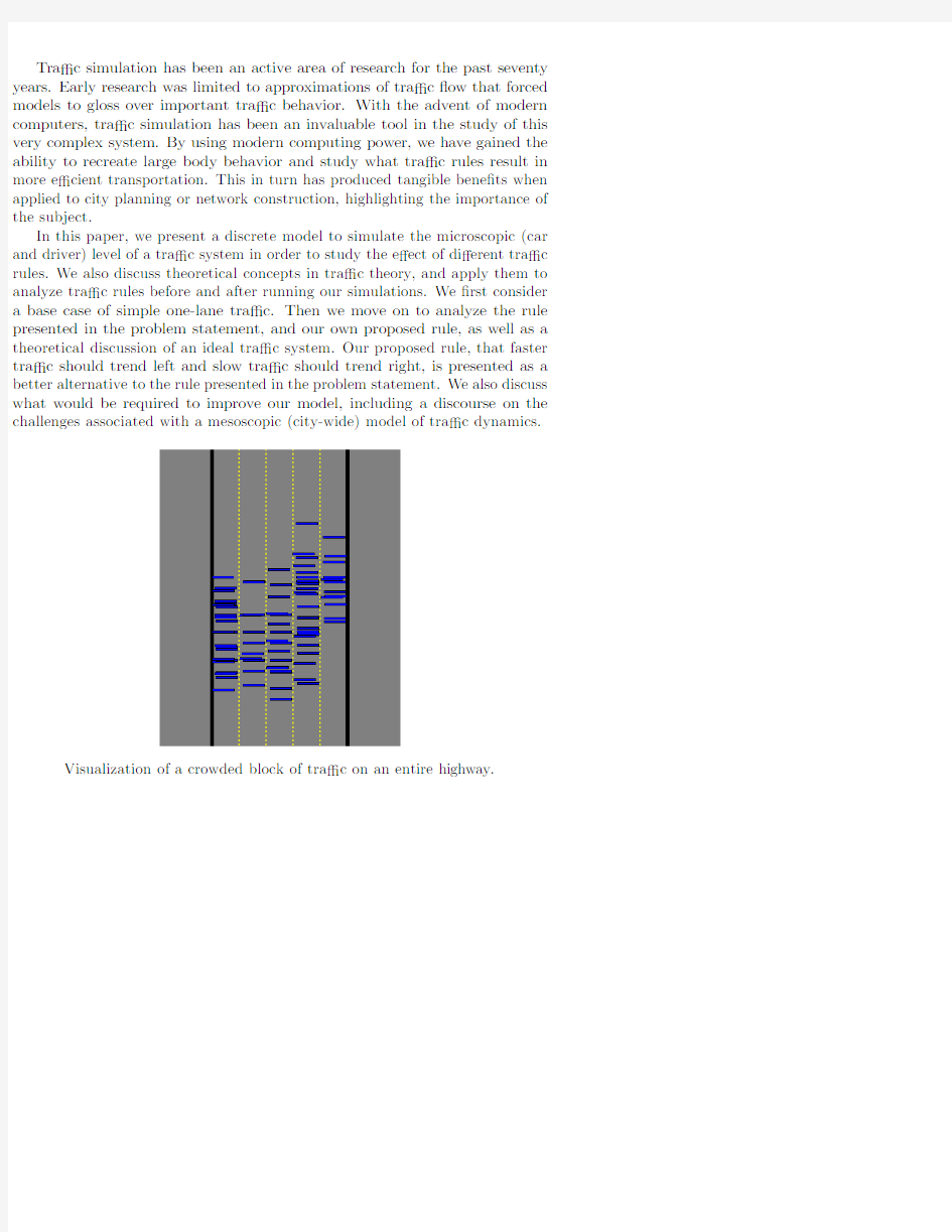
In this paper,we present a discrete model to simulate the microscopic(car and driver)level of a tra c system in order to study the e?ect of di?erent tra c rules.We also discuss theoretical concepts in tra c theory,and apply them to analyze tra c rules before and after running our simulations.We?rst consider a base case of simple one-lane tra c.Then we move on to analyze the rule presented in the problem statement,and our own proposed rule,as well as a theoretical discussion of an ideal tra c system.Our proposed rule,that faster tra c should trend left and slow tra c should trend right,is presented as a better alternative to the rule presented in the problem statement.We also discuss what would be required to improve our model,including a discourse on the challenges associated with a mesoscopic(city-wide)model of tra c dynamics.

Visualization of a crowded block of tra c on an entire highway.

Beating the Tra c:An Analysis of Alternative

Tra c Rules

Control#29221

February10,2014

Page1of13Control#29221

Contents

1Introduction2

1.1Outline of Approach (2)

1.2Assumptions (2)

2Background3

2.1De?nitions (3)

2.2Introduction to our Model (4)

3Analysis of the Standard Maneuver6

3.1Theoretical Approach (6)

3.2Computational Approach (6)

4Analysis of a New Rule8

4.1Theoretical Approach (8)

4.2Computational Approach (8)

5Modi?cations and Extensions10

5.1Driving on the Left Side (10)

5.2Safety Trade-o? (10)

5.3Varied Speed Limits (11)

5.4An Ideal System (11)

6Conclusion11 7References13

Page2of13Control#29221

1Introduction

1.1Outline of Approach

In this paper we will present a discrete model for small scale tra c?ow.We de?ne small scale tra c to be tra c where the signi?cant dynamics are determined by actions of individual drivers,as opposed to large scale where one might just look at di?erential equations governing the?ow,with little or no interaction from individuals who make up that?ow.We present some tra c theory de?nitions and construct a discretized model of a highway under varying tra c load and varying rules for how drivers behave.The basic structure of each model is the same,we have a road which has been discretized into4-foot sections,each car will take up4of these sections.Each road has a varying number of lanes,from1 to5.Cars are placed in positions in each lane and we then take time steps of 1second.In each time step every driver will make a choice about whether to switch lanes or to maintain,decrease,or increase their velocity.When sequenced together we have information about positions and velocities unique to each car in our model for the entire time we run the model.We will then analyze these results and compare di?erent tra c rules in order to get a better understanding of why certain rules are more e cient at allowing tra c?ow,while highlighting the?aws in others.

1.2Assumptions

?In our models we assume that the speed limit is approximately 71miles per hour.

This corresponds to a velocity of26units per time step as we use4foot units and1second time steps.Highway speeds vary from55to85miles per hour on average depending on population and road size.In a sparsely populated area with a reasonable sized highway75miles per hour seems to be a good average.

?We assume that no driver speeds,

For simplicity sake,this is of course an untrue assumption,but when determining the usefulness of a law,we should assume that all other laws relating are followed,otherwise our analysis would be of the system of laws, not an objective evaluation of any single law.In order to not lock cars out of being able to merge,we allowed drivers to merge even if they would be bumper to bumper.This helps to simulate the fact that in reality,drivers will often allow others to merge,while our model isn’t that interactive.?We assume that drivers are making decisions according to our rules and reacting within one second.

We assume that the maximum breaking speed is 28ft/s2,and the maxi-mum acceleration is4ft/s2,this is based on information from the United States Department of Transportation.The?nal assumption we made was

Page3of13Control#29221 that if two cars are in a collision then they are removed from the road.In reality,they would probably pull over,but in our model they are instantly removed from the simulation to reduce complexity.

2Background

2.1De?nitions

We will start by de?ning several statistics from tra c theory following the standards introduced in[4].The?rst important quantity is the“?ow”of a highway.Intuitively we want to talk about the amount of tra c that goes across a highway.To calculate the?ow,we imagine taking a tiny slice of road across the lanes of our highway.Then,we start a stopwatch wait and count the number of cars that travel over this slice.Once our stopwatch hits a predetermined value (called?in our paper),we stop counting the cars.The ratio of cars crossed to time elapsed is our value for q,the“?ow”.However,our tra c model is discrete in nature,so both our“tiny”slice of road and our“tiny”slice in time are actually sizable.This means that in order to achieve good values for q,we must average the?ow over a time period much longer than our discretization.

There is also another critical quantity we need to introduce from tra c theory, called the“space-averaged density”.The letter reserved for this is usually k, and this notation is used throughout the rest of our paper.k is the number of vehicles in a given strip of highway.Again,imagine placing a marker at some point x1,and another marker further down the road at some point x2.Then,at a particular time,we count the number of cars between the two markers.The ratio of counted cars to the distance of our markers is k.k is a quantity,like q, that makes sense in an averaged context.You could imagine moving the markers around and getting di?erent values for k due to the fact that cars are discrete, but this e?ect is diminished if we only consider large stretches of highway.

q and k can,and should,vary over a highway,especially if certain regions are heavier with tra c than others,such as a merging lane or an accident.To get an idea of how q changes as a function of k(the density of tra c),we need to average q over the highway.This is done by taking slices100units apart,ranging from our“start”of the highway x=0,to the x coordinate of the furthest vehicle on highway,rounded up to the nearest100.This last value,divided by100 we call N,since it corresponds to the number of slices on the highway for our calculation.

q=1

N X i=1...N Number of cars passing through x i

?

=q=

1

N X i=1...N100i?.

Since?is independent of the summand,we can factor it out.Additionally,we can re-express the sum using the fact that there are a?nite number of cars, labelled from1to M.So,

q=

1

N?X i=1...N X j=1...M bool(car j passes through x i)

Page4of13Control#29221 Where bool(A)is1if A is true and0if A is false.This may seem daunting, however,our computer simulation has the handy property of recording the?rst and last positions of every car.So,given any slice of highway x i,if a particular car starts before the slice at t=0,and ends up after the slice at t=?,then we know for a fact that it passed through the slice.This converts our rather ugly looking sum into the much more palatable form of

q=

1

100N?X j=1...M b x final x start c

where j runs over the indices of the cars.

Our simulation of one lane tra c uses random assignments in position and

velocity to accurately re-create tra c conditions.To account for the possible

discrepancy in car density due to this feature,we average car density over the

highway using a similar procedure to the one above.The space averaged density

k at a particular time is simply the number of cars on the highway behind the

furthest car and in front of the car furthest behind.So,the space averaged

density k is(#of cars)/(x most x least).However,the space averaged density varies in time,so to establish a proper relationship between q and k,we need to

time average k as well.This is done by averaging k over equal intervals of one

hundred seconds,so

k=1

6

600

X t=100#of cars at t

x most x least

where x most and x least are both functions of time,since the car in front will continue to move,as will the car in the back,and not necessarily at the same rates.For our single lane analysis,the car in front will remain in that position, whereas in multi-lane models further in our paper the car identity is not conserved. Additionally,in continuous tra c stream models x least can simply be replaced by0,since more cars will constantly be added during every time step near the start of the highway.

2.2Introduction to our Model

Here we will introduce a model for tra c in one lane.This is a very simple case as we won’t have to consider lane switching,each car on the road will only worry about the behavior of the car directly in front of it.Here is a?ow chart of the decisions:

Page5of13Control#29221

As a car in the system,your?rst choice is whether or not the follow distance you are currently maintaining is enough.We chose three car lengths to be the target follow distance,this is based on recommendations by driver’s manuals in the United States.We determine this by estimating both where we will be in one time step,and where the car in front of us will be.If this distance does not have the required spacing,we attempt to slow down until we achieve the safe spacing.If that spacing is achieved then the only other thing we,as a car,worry about is the speed limit.If we are below the speed limit,we accelerate,if we are at the speed limit then we continue on our journey.Note that in this model it is impossible to go above the speed limit as we only increase our velocity if we are below the speed limit,every other case maintains or loses velocity.With this model we can observe some of the statistics described above.

If tra c is light enough that any given car can safely reach the speed limit then we expect to see the?ow,q,increase as the density k increases until the amount of cars begins to a?ect the ability of drivers to safely reach the speed limit.After this point we expect to see a decline in q all the way to0,at which tra c is gridlocked.

As we can see in Figure1,the?ow rate,q,has a peak in the middle.This is the zone where tra c isn’t dense enough to a?ect tra c patterns.After a certain point this value quickly drops o?as the density of the highway approaches gridlock.This con?rms our analysis of the simple model and seems to agree with reality as far as we can tell.

Page6of13Control#29221

Figure1:Simulated results of tra c?ow vs density in single lane tra c

3Analysis of the Standard Maneuver

3.1Theoretical Approach

The standard maneuver is the rule stating that a driver may only use the left lane to pass someone,if they are not passing,then they should move back to the right lane.Intuitively this means that when there are a lot of lanes and a lot of tra c,the leftmost lanes will be underused and cause unnecessary congestion in the right lanes,this will be due to the fact that no one is using the left lanes for travel,but only to pass a slower car in front of themselves.Our initial thought was that this rule seemed very ine cient.In this model if a faster car approaches a slower car,if it is unable to immediately switch lanes to start passing,it will have to slow down.That slowing will propagate backward down the lane until a car is able to begin the maneuver.

3.2Computational Approach

In our computational approach to analyzing this rule,we made several changes to the basic model outlined in the previous section.We consider n lanes instead of only one,which introduces the possibility of cars switching lanes.This leads to a lengthy decision tree that must be gone through for each car in each time step.The general?ow is as follows:

Page7of13Control#29221

Unlike in the simple model,here we must consider an extra dimension,more lanes,and adherence to a new rule.As a car in the model,the?rst choice we will make is whether or not we want to pass the car in front of us.If they are moving at a lower velocity than us,we assume that we do want to pass them.If we want to pass them,then we?rst check if it is okay to merge left.If so,we can go ahead and change lanes,but if not we will assume that we cannot pass and according to the rule,we must attempt to get back into the right lane.So we check whether or not that is safe.If it is not,we simplify back to the case in the simple model where we only care about not getting too close to the car in front of us and maintaining the speed limit.

The expected behavior of this system is slightly di?erent than the simple model.In the case where there is low enough tra c density,we expect all tra c to be in the right lane and the system to behave like the one lane simple case. However,as we increase the density,instead of seeing a decrease in?ow where we would in the simple model,we expect to see?ow increase beyond this point because faster tra c will start to spill over into the left lanes until they can merge back.This will mean that the?ow can handle a denser system for longer. Eventually we will see a gridlock steady state when all of the lanes get?lled up, but that will take signi?cantly longer than in the simple model.

In Figure2we can see that the peak q value is higher than that in the simple model.This is because tra c is able to move more smoothly when merging is allowed.Tra c which would get stuck can choose to pass the obstruction and continue at a higher rate.We notice that the k value for which the system starts to decline is very similar to the simple model,meaning that it doesn’t handle a larger density of tra c than the simple model,but an equal amount,only more e ciently.

Page8of13Control#29221

Figure2:Simuated results for?ow vs density using“standard maneuver”rule 4Analysis of a New Rule

4.1Theoretical Approach

The motivation for this new rule was that driver’s inherently have a speed at which they are comfortable moving,if we group these drivers together,they can continue at that speed,this removes the e?ect of one slow down causing a ripple e?ect backwards down the lane.Faster tra c will move left,while slower tra c will move right.It is a very simple rule that drivers can easily understand.One potential downside of this model is that changing lanes either to the right or the left could become dangerous if the change in speed is drastically di?erent as a driver would have to either speed up or slow down in order to pass.

4.2Computational Approach

The?ow chart for our proposed rule is as follows:

Page9of13Control#29221

In this model each car has a target speed,either at,above,or below the speed limit.The further left a lane is,the higher average speed it has.Faster cars will want to move left and slower cars will want to move right.The decision in any time set for any given car starts by asking whether the car is in the optimal lane for its speed,in this case,the lane whose average speed is closest to the target speed.If they are,they use the behavior from the simple model.If they aren’t, then then will check and attempt to merge in the direction which changes their speed to be closer to their target speed.Given a section of tra c,we expect this model to have a fairly chaotic initial stage,then converge to a steady state behavior when each car is in it’s ideal lane.Overall we expect this to be more e cient in terms of tra c?ow than the standard maneuver because it will allow some tra c to move faster and will reduce the amount of slowing generated when a faster vehicle approaches a slower one and has to begin to slow down itself,which will then chain backwards to each car behind them for some depth of cars.In our case we use?ve lanes,the three left-most lanes are increments above the speed limit,the second from the right is at the speed limit,and the right lane is slightly below the speed limit.

Speci?cally we can expect that this rule will have much greater?ow than if we used the simple model in every lane of a multi-lane highway.In the case where we have multiple simple models the?ow will be limited by the speed limit and by any driver who drives below that.After the initial chaotic behavior of our new model,when every driver has found their ideal lane,we can expect a steady state where four of the lanes are moving at a rate faster than lanes of the simple model,and the?fth is moving slightly slower.Overall this translates to a higher q when density is high.

In Figure3we can see that the peak q value is higher and it occurs at a higher k value.This shows that the rule can handle a higher number of cars

Page10of13Control#29221

Figure3:Simulated results of tra c?ow vs density using new rule while still operating at a high rate.This con?rms what we would expect from this rule.The tra c merges a lot in the?rst time steps,then it settles into a highly e cient pattern where more lanes are able to move quicker.

5Modi?cations and Extensions

5.1Driving on the Left Side

Our model is not dependent on orientation.If we simply?ip the orientation of the drivers and the roads we get an identical problem,di?erent only in direction.

5.2Safety Trade-o?

Of course,a natural concern for any heuristic about driving is safety.According to the World Health Organization,road tra c injuries caused an estimated1.24 million deaths worldwide in the year2010.Our models take into account the potential for automobiles to hit each other.On a?ve lane highway with a speed limit of71miles per hour,due to limitations of our model,we experience a small amount of collisions immediately,but this number quickly goes to zero when we reach a steady state.In all of the tra c rules that we modeled,collisions were demonstrated to occur at a higher incidence when more complicated behavior such as changing lanes,or accelerating more aggressively was prevalent.This is to be expected,compared to the much simpler case of several drivers driving in a single lane,where intuitively,we would expect that collisions are more easily preventable.Our models re?ect this by producing less car collisions in the simple single lane situation,than are produced in more complicated multi-lane situation.

Page11of13Control#29221

5.3Varied Speed Limits

When we run our models with higher than average speed limits,we notice a dramatic increase in collisions.This is to be expected,as an increase in speed leads to more di culty slowing down in the event of a change in velocity of the ?ow.Cars can only brake at a certain rate,if we go fast enough that this doesn’t signi?cantly impact the distance we will travel in the seconds before a collision, then collisions become very hard to avoid.This is made even worse in models where cars actively switch lanes,the combination of high speeds and the fact that our model has limited ability to predict the safety of a merge gives us a frightening fatality rate for even a small number of drivers.However there are certain systems where extremely high speeds would only improve the?ow. 5.4An Ideal System

In an ideal system the whole tra c system is controlled by an intelligent system. Under this assumption we can have cars moving at a much faster speed and have safety be una?ected.Imagine a road where every car was controlled by a central computer.This computer knows the position and velocity of each car and can adjust the acceleration of any car.The biggest safety hazard on highways is when people travel at di?erent speeds,this can be removed from the equation when a computer can have each car in the system travel at precisely the same speed.In a line of cars all moving at the same rate,there is no chance of a collision.

Taking this system a step further we can imagine that to handle merging the computer could slow down portions of tra c by a small,fractional amount, in order to create gaps for more cars to merge into the system.When done by a centralized power like this,reaction,overreaction,and any propagation of slowing can be minimized.The e?ect of propagation can be absorbed in smaller and smaller amounts until it is unnoticeable to a human observer.Under these conditions we can reach what would be a theoretical maximal tra c?ow,limited locally only by the top speed of the slowest vehicle and globally by the top speed of a car.

In such a system the?ow q is maximized as there is no slow down when adding more cars,the curve of k vs.q will have a plateaued maximum because once we reach saturation,adding more cars won’t increase the?ow,but it won’t decrease it either.The only limit on q is on how perfect the control is and the physical capacities of cars.

6Conclusion

In this paper we examined a discrete model for modeling tra c patterns based on individual decisions of drivers.This is a much di?erent problem than examining the system from a macroscopic point of view,however both methods are useful for examining di?erent properties.We chose to focus on the microscopic system because we are better able to see how rules a?ect individual drivers and can see

Page12of13Control#29221 trends on tra c as a whole.We compared di?erent rules to the base case of a simple model where cars don’t switch lanes and only worry about following the speed limit,and not hitting the car in front of them.

The?rst rule we analyzed stated that a driver should remain in the right lane unless they are passing another slower car.We called this the standard model.We found that this was more e?ective than the base case.Faster tra c was able to escape a slower?ow and spill into additional lanes when it needed to,which allowed for a reduction in the amount of slowing observed when the road started to become crowded.

The second rule was our proposed rule.This rule dictated that faster cars move to the left and slower cars move to the right.This creates an ideal lane for each driver based on the speed they want to travel.After the system settles and each driver?nds their preferred lane,the?ow is much improved over both the simple and standard model.This was due to the fact that in the steady state more lanes were moving faster than in the simple or standard case.Faster tra c was not impeded by slower tra c,which increased the overall?ow at high densities.In the steady state,this model is also safer.Tra c is at its safest when every vehicle is traveling at the same speed,this reduces the need for reaction due to a driver having to slow down for tra c and it is impossible to run into another driver unless you are switching lanes incorrectly or there is an unforeseen accident which requires a change in speed.In each of the other models we have tra c which wants to move faster,but cannot due to a slower car.They are then required to slow down,which puts them and everyone behind them at risk because it requires action on behalf of other drivers.

We found that our model is independent of the side of the road it is standard to drive on;simply changing the orientation is a su cient modi?cation.If we consider an ideal system,we can imagine that it is an improved version of our proposed rule,where every lane is as fast the vehicles can safely handle,and merging is no longer a threat to safety because it can be precisely and centrally controlled.

We can think of several extensions and improvements to our model,the ?rst being to increase the scale and accuracy.We were limited in our time and hardware,but ideally we would run a longer simulation with many more cars and remove most of the simplifying assumptions outlined earlier.This would give us a better idea of the dynamics of each scenario.It is also possible to extend the discussion to a continuous system governed by partial di?erential equations,this would give a clearer picture of large scale phenomena,but is poor at describing the behavior of individual drivers.There are even models in the current literature that combine the macroscopic and microscopic scales into a mesoscopic model. These are very involved models,and are similar to computing gas dynamics by the interactions of individual particles.Given adequate resources,these types of models could be very informative and provide much more in-depth and accurate results than either the macro-or micro-scopes could.

Page13of13Control#29221

7References

[1]Ding Ding,Modeling and simulation of highway traf-

?c using a cellular automaton approach https://www.360docs.net/doc/e77469106.html,/smash/get/diva2:483914/FULLTEXT01.pdf,2011.

[2]Serge Hoogendoorn and Victor Knoop,Tra c?ow theory and modelling

http://www.victorknoop.eu/research/papers/chapter vanwee.pdf,2012. [3]Fred L.Hall,Tra c Stream Characteristics

https://https://www.360docs.net/doc/e77469106.html,/publications/research/operations/tft/chap2.pdf, 1992.

[4]M.J.Lighthill and G.B.Whitham On kinematic waves II,A theory of tra c

?ow on long crowded roads1955