pid控制外文加中文文献

PID controller
From Wikipedia, the free encyclopedia
A proportional–integral–derivative controller (PID controller) is a generic .control loop feedback mechanism widely used in industrial control systems.
A PID controller attempts to correct the error between a measured process variable and a desired setpoint by calculating and then outputting a corrective action that can adjust the process accordingly.
The PID controller calculation (algorithm) involves three separate parameters; the Proportional, the Integral and Derivative values. The Proportional value determines the reaction to the current error, the Integral determines the reaction based on the sum of recent errors and the Derivative determines the reaction to the rate at which the error has been changing. The weightedsum of these three actions is used to adjust the process via a control element such as the position of a control valve or the power supply of a heating element.By "tuning" the three constants in the PID controller algorithm the PID can provide control action designed for specific process requirements. The response of the controller can be described in terms of the responsiveness of the controller to an error, the degree to which the controller overshoots the setpoint and the degree of system oscillation. Note that the use of the PID algorithm for control does not guarantee optimal control of the system or system stability.
Some applications may require using only one or two modes to provide the appropriate system control. This is achieved by setting the gain of undesired control outputs to zero. A PID controller will be called a PI, PD, P or I controller in the absence of the respective control actions. PI controllers are particularly common, since derivative action is very sensitive to measurement noise, and the absence of an integral value may prevent the system from reaching its target value due to the control action.
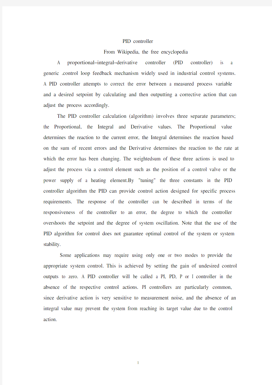
A block diagram of a PID controller
Note: Due to the diversity of the field of control theory and application, many naming conventions for the relevant variables are in common use.
1.Control loop basics
A familiar example of a control loop is the action taken to keep one's shower water at the ideal temperature, which typically involves the mixing of two process streams, cold and hot water. The person feels the water to estimate its temperature. Based on this measurement they perform a control action: use the cold water tap to adjust the process. The person would repeat this input-output control loop, adjusting the hot water flow until the process temperature stabilized at the desired value.
Feeling the water temperature is taking a measurement of the process value or process variable (PV). The desired temperature is called the setpoint (SP). The output from the controller and input to the process (the tap position) is called the manipulated variable (MV). The difference between the measurement and the setpoint is the error (e), too hot or too cold and by how much.As a controller, one decides roughly how much to change the tap position (MV) after one determines the temperature (PV), and therefore the error. This first estimate is the equivalent of the proportional action of a PID controller. The integral action of a PID controller can be thought of as gradually adjusting the temperature when it is almost right. Derivative action can be thought of as noticing the water temperature is getting hotter or colder, and how fast, and taking that into account when deciding how to adjust the tap.Making a change that is too large when the error is small is equivalent to a high gain controller and will lead to
overshoot. If the controller were to repeatedly make changes that were too large and repeatedly overshoot the target, this control loop would be termed unstable and the output would oscillate around the setpoint in either a constant, growing, or decaying sinusoid. A human would not do this because we are adaptive controllers, learning from the process history, but PID controllers do not have the ability to learn and must be set up correctly. Selecting the correct gains for effective control is known as tuning the controller.
If a controller starts from a stable state at zero error (PV = SP), then further changes by the controller will be in response to changes in other measured or unmeasured inputs to the process that impact on the process, and hence on the PV. Variables that impact on the process other than the MV are known as disturbances and generally controllers are used to reject disturbances and/or implement setpoint changes. Changes in feed water temperature constitute a disturbance to the shower process.
In theory, a controller can be used to control any process which has a measurable output (PV), a known ideal value for that output (SP) and an input to the process (MV) that will affect the relevant PV. Controllers are used in industry to regulate temperature, pressure, flow rate, chemical composition, speed and practically every other variable for which a measurement exists. Automobile cruise control is an example of a process which utilizes automated control.
Due to their long history, simplicity, well grounded theory and simple setup and maintenance requirements, PID controllers are the controllers of choice for many of these applications.
2.PID controller theory
Note: This section describes the ideal parallel or non-interacting form of the PID controller. For other forms please see the Section "Alternative notation and PID forms".
The PID control scheme is named after its three correcting terms, whose sum constitutes the manipulated variable (MV). Hence:
where Pout, Iout, and Dout are the contributions to the output from the PID controller from each of the three terms, as defined below.
2.1. Proportional term
The proportional term makes a change to the output that is proportional to the current error value. The proportional response can be adjusted by multiplying the error by a constant Kp, called the proportional gain.
The proportional term is given by:
Where
Pout: Proportional output
Kp: Proportional Gain, a tuning parameter
e: Error = SP ? PV
t: Time or instantaneous time (the present)
Change of response for varying KpA high proportional gain results in a large change in the output for a given change in the error. If the proportional gain is too high, the system can become unstable (See the section on Loop Tuning). In contrast, a small gain results in a small output response to a large input error, and a less responsive (or sensitive) controller. If the proportional gain is too low, the control action may be too small when responding to system disturbances.
In the absence of disturbances, pure proportional control will not settle at its target value, but will retain a steady state error that is a function of the proportional gain and the process gain. Despite the steady-state offset, both tuning theory and industrial practice indicate that it is the proportional term that should contribute the bulk of the output change.
2.2.Integral term
The contribution from the integral term is proportional to both the magnitude of the error and the duration of the error. Summing the instantaneous error over time (integrating the error) gives the accumulated offset that should have been corrected previously. The accumulated error is then multiplied by the integral gain and added to the controller output. The magnitude of the contribution of the integral term to the overall control action is determined by the integral gain, Ki.
The integral term is given by:
Change of response for varying KiWhere
Iout: Integral output
Ki: Integral Gain, a tuning parameter
e: Error = SP ? PV
τ: Time in the past contributing to the integral response
The integral term (when added to the proportional term) accelerates the
movement of the process towards setpoint and eliminates the residual steady-state error that occurs with a proportional only controller. However, since the integral term is responding to accumulated errors from the past, it can cause the present value to overshoot the setpoint value (cross over the setpoint and then create a deviation in the other direction). For further notes regarding integral gain tuning and controller stability, see the section on loop tuning.
2.3 Derivative term
The rate of change of the process error is calculated by determining the slope of the error over time (i.e. its first derivative with respect to time) and multiplying this rate of change by the derivative gain Kd. The magnitude of the contribution of the derivative term to the overall control action is termed the derivative gain, Kd.
The derivative term is given by:
Change of response for varying KdWhere
Dout: Derivative output
Kd: Derivative Gain, a tuning parameter
e: Error = SP ? PV
t: Time or instantaneous time (the present)
The derivative term slows the rate of change of the controller output and this effect is most noticeable close to the controller setpoint. Hence, derivative control is
used to reduce the magnitude of the overshoot produced by the integral component and improve the combined controller-process stability. However, differentiation of a signal amplifies noise and thus this term in the controller is highly sensitive to noise in the error term, and can cause a process to become unstable if the noise and the derivative gain are sufficiently large.
2.4 Summary
The output from the three terms, the proportional, the integral and the derivative terms are summed to calculate the output of the PID controller. Defining u(t) as the controller output, the final form of the PID algorithm is:
and the tuning parameters are
Kp: Proportional Gain - Larger Kp typically means faster response since the
larger the error, the larger the Proportional term compensation. An excessively large proportional gain will lead to process instability and oscillation.
Ki: Integral Gain - Larger Ki implies steady state errors are eliminated quicker. The trade-off is larger overshoot: any negative error integrated during transient response must be integrated away by positive error before we reach steady state.
Kd: Derivative Gain - Larger Kd decreases overshoot, but slows down transient response and may lead to instability due to signal noise amplification in the differentiation of the error.
3. Loop tuning
If the PID controller parameters (the gains of the proportional, integral and derivative terms) are chosen incorrectly, the controlled process input can be unstable, i.e. its output diverges, with or without oscillation, and is limited only by saturation or mechanical breakage. Tuning a control loop is the adjustment of its control parameters (gain/proportional band, integral gain/reset, derivative gain/rate) to the optimum values for the desired control response.
The optimum behavior on a process change or setpoint change varies depending on the application. Some processes must not allow an overshoot of the process
variable beyond the setpoint if, for example, this would be unsafe. Other processes must minimize the energy expended in reaching a new setpoint. Generally, stability of response (the reverse of instability) is required and the process must not oscillate for any combination of process conditions and setpoints. Some processes have a degree of non-linearity and so parameters that work well at full-load conditions don't work when the process is starting up from no-load. This section describes some traditional manual methods for loop tuning.
There are several methods for tuning a PID loop. The most effective methods generally involve the development of some form of process model, then choosing P, I, and D based on the dynamic model parameters. Manual tuning methods can be relatively inefficient.
The choice of method will depend largely on whether or not the loop can be taken "offline" for tuning, and the response time of the system. If the system can be taken offline, the best tuning method often involves subjecting the system to a step change in input, measuring the output as a function of time, and using this response to determine the control parameters.
Choosing a Tuning Method
MethodAdvantagesDisadvantages
Manual TuningNo math required. Online method.Requires experienced
personnel.
Ziegler–NicholsProven Method. Online method.Process upset, some
trial-and-error, very aggressive tuning.
Software ToolsConsistent tuning. Online or offline method. May include
valve and sensor analysis. Allow simulation before downloading.Some cost
and training involved.
Cohen-CoonGood process models.Some math. Offline method. Only good for first-order processes.
3.1 Manual tuning
If the system must remain online, one tuning method is to first set the I and D values to zero. Increase the P until the output of the loop oscillates, then the P should
be left set to be approximately half of that value for a "quarter amplitude decay" type response. Then increase D until any offset is correct in sufficient time for the process. However, too much D will cause instability. Finally, increase I, if required, until the loop is acceptably quick to reach its reference after a load disturbance. However, too much I will cause excessive response and overshoot. A fast PID loop tuning usually overshoots slightly to reach the setpoint more quickly; however, some systems cannot accept overshoot, in which case an "over-damped" closed-loop system is required, which will require a P setting significantly less than half that of the P setting causing oscillation.
Effects of increasing parameters
Parameter Rise Time shootSettling Time S.S. Error Kp Decrease Increase Small Change Decrease
Ki Decrease Increase Increase Eliminate
Kd Small Decrease Decrease Decrease None
3.2Ziegler–Nichols method
Another tuning method is formally known as the Ziegler–Nichols method, introduced by John G. Ziegler and Nathaniel B. Nichols. As in the method above, the I and D gains are first set to zero. The "P" gain is increased until it reaches the "critical gain" Kc at which the output of the loop starts to oscillate. Kc and the oscillation period Pc are used to set the gains as shown:
Ziegler–Nichols method
Kp Ki Kd
Control
Type
P 0.5 Kc - -
PI 0.45Kc 1.2 Kp /Pc -
PID 0.6 Kc 2Kp / Pc KpPc / 8
3.3 PID tuning software
Most modern industrial facilities no longer tune loops using the manual
calculation methods shown above. Instead, PID tuning and loop optimization software are used to ensure consistent results. These software packages will gather the data, develop process models, and suggest optimal tuning. Some software packages can even develop tuning by gathering data from reference changes.
Mathematical PID loop tuning induces an impulse in the system, and then uses the controlled system's frequency response to design the PID loop values. In loops with response times of several minutes, mathematical loop tuning is recommended, because trial and error can literally take days just to find a stable set of loop values. Optimal values are harder to find. Some digital loop controllers offer a self-tuning feature in which very small setpoint changes are sent to the process, allowing the controller itself to calculate optimal tuning values.
Other formulas are available to tune the loop according to different performance criteria.
4 Modifications to the PID algorithm
The basic PID algorithm presents some challenges in control applications that have been addressed by minor modifications to the PID form.One common problem resulting from the ideal PID implementations is integral
windup. This can be addressed by:
Initializing the controller integral to a desired value
Disabling the integral function until the PV has entered the controllable region Limiting the time period over which the integral error is calculated
Preventing the integral term from accumulating above or below pre-determined bounds
Many PID loops control a mechanical device (for example, a valve). Mechanical maintenance can be a major cost and wear leads to control degradation in the form of either stiction or a deadband in the mechanical response to an input signal. The rate of mechanical wear is mainly a function of how often a device is activated to make a change. Where wear is a significant concern, the PID loop may have an output deadband to reduce the frequency of activation of the output (valve). This is accomplished by modifying the controller to hold its output steady if the change
would be small (within the defined deadband range). The calculated output must leave the deadband before the actual output will change.The proportional and derivative terms can produce excessive movement in the output when a system is subjected to an instantaneous "step" increase in the error, such as a large setpoint change. In the case of the derivative term, this is due to taking the derivative of the error, which is very large in the case of an instantaneous step change.
5. Limitations of PID control
While PID controllers are applicable to many control problems, they can perform poorly in some applications.PID controllers, when used alone, can give poor performance when the PID loop gains must be reduced so that the control system does not overshoot, oscillate or "hunt" about the control setpoint value. The control system performance can be improved by combining the feedback (or closed-loop) control of a PID controller with feed-forward (or open-loop) control. Knowledge about the system (such as the desired acceleration and inertia) can be "fed forward" and combined with the PID output to improve the overall system performance. The feed-forward value alone can often provide the major portion of the controller output. The PID controller can then be used primarily to respond to whatever difference or "error" remains between the setpoint (SP) and the actual value of the process variable (PV). Since the feed-forward output is not affected by the process feedback, it can never cause the control system to oscillate, thus improving the system response and stability.
For example, in most motion control systems, in order to accelerate a mechanical load under control, more force or torque is required from the prime mover, motor, or actuator. If a velocity loop PID controller is being used to control the speed of the load and command the force or torque being applied by the prime mover, then it is beneficial to take the instantaneous acceleration desired for the load, scale that value appropriately and add it to the output of the PID velocity loop controller. This means that whenever the load is being accelerated or decelerated, a proportional amount of force is commanded from the prime mover regardless of the feedback value. The PID loop in this situation uses the feedback information to effect any increase or decrease of the combined output in order to reduce the remaining difference between the
process setpoint and the
feedback value. Working together, the combined open-loop feed-forward controller and closed-loop PID controller can provide a more responsive, stable and reliable control system.
Another problem faced with PID controllers is that they are linear. Thus, performance of PID controllers in non-linear systems (such as HV AC systems) is variable. Often PID controllers are enhanced through methods such as PID gain scheduling or fuzzy logic. Further practical application issues can arise from instrumentation connected to the controller. A high enough sampling rate, measurement precision, and measurement accuracy are required to achieve adequate control performance.
A problem with the Derivative term is that small amounts of measurement or process noise can cause large amounts of change in the output. It is often helpful to filter the measurements with a low-pass filter in order to remove higher-frequency noise components. However, low-pass filtering and derivative control can cancel each other out, so reducing noise by instrumentation means is a much better choice. Alternatively, the differential band can be turned off in many systems with little loss of control. This is equivalent to using the PID controller as a PI controller.
6. Cascade control
One distinctive advantage of PID controllers is that two PID controllers can be used together to yield better dynamic performance. This is called cascaded PID control. In cascade control there are two PIDs arranged with one PID controlling the set point of another. A PID controller acts as outer loop controller, which controls the primary physical parameter, such as fluid level or velocity. The other controller acts as inner loop controller, which reads the output of outer loop controller as set point, usually controlling a more rapid changing parameter, flowrate or accelleration. It can be mathematically proved that the working frequency of the controller is increased and the time constant of the object is reduced by using cascaded PID controller.[vague]
7. Physical implementation of PID control
In the early history of automatic process control the PID controller was implemented as a mechanical device. These mechanical controllers used a lever, spring and a mass and were often energized by compressed air. These pneumatic controllers were once the industry standard.Electronic analog controllers can be made from a solid-state or tube amplifier, a capacitor and a resistance. Electronic analog PID control loops were often found within more complex electronic systems, for example, the head positioning of a disk drive, the power conditioning of a power supply, or even the movement-detection circuit of a modern seismometer. Nowadays, electronic controllers have largely been replaced by digital controllers implemented with microcontrollers or FPGAs.
Most modern PID controllers in industry are implemented in software in programmable logic controllers (PLCs) or as a panel-mounted digital controller. Software implementations have the advantages that they are relatively cheap and are flexible with respect to the implementation of the PID algorithm.
8.Alternative nomenclature and PID forms
8.1 Pseudocode
Here is a simple software loop that implements the PID algorithm:
previous_error = 0
start:
error = setpoint - actual_position
P = Kp * error
I = I + Ki * error * dt
D = (Kd / dt) * (error - previous_error)
output = P + I + D
previous_error = error
wait(dt)
goto start
8.2 Ideal versus standard PID form
The form of the PID controller most often encountered in industry, and the one most relevant to tuning algorithms is the "standard form". In this form the Kp gain is applied to the Iout, and Dout terms, yielding:
Where
Ti is the Integral Time
Td is the Derivative Time
In the ideal parallel form, shown in the Controller Theory section
the gain parameters are related to the parameters of the standard form
through
and Kd = KpTd. This parallel form, where the parameters are treated as simple gains, is the most general and flexible form. However, it is also the form where the parameters have the least physical interpretation and is generally reserved for theoretical treatment of the PID controller. The "standard" form, despite being slightly more complex mathematically, is more common in industry.
8.3Laplace form of the PID controller
Sometimes it is useful to write the PID regulator in Laplace transform form:
Having the PID controller written in Laplace form and having the transfer function of the controlled system, makes it easy to determine the closed-loop transfer function of the system.
8.4Series / interacting form
Another representation of the PID controller is the series, or "interacting" form. This form essentially consists of a PD and PI controller in series, and it made early (analog) controllers easier to build. When the controllers later became digital, many kept using the interacting form.
[edit] References
Liptak, Bela (1995). Instrument Engineers' Handbook: Process Control. Radnor, Pennsylvania: Chilton Book Company, 20-29. ISBN 0-8019-8242-1.
Van, Doren, Vance J. (July 1, 2003). "Loop Tuning Fundamentals". Control Engineering. Red Business Information.
Sellers, David. An Overview of Proportional plus Integral plus Derivative Control and Suggestions for Its Successful Application and Implementation (PDF). Retrieved on 2007-05-05.
Articles, Whitepapers, and tutorials on PID control
Graham, Ron (10/03/2005). FAQ on PID controller tuning. Retrieved on
2007-05-05.
PID控制器
比例积分微分控制器(PID调节器)是一个控制环,广泛地应用于工业控制系统里的反馈机制。PID控制器通过调节给定值与测量值之间的偏差,给出正确的调整,从而有规律地纠正控制过程。
PID控制器算法涉及到三个部分:比例,积分,微分。比例控制是对当前偏差的反应,积分控制是基于新近错误总数的反应,而微分控制则是基于错误变化率的反应。这三种控制的结合可用来调节过程系统,例如调节阀的位置,或者加热系统的电源调节。根据具体的工艺要求,通过PID控制器的参数整定,从而提供调节作用。控制器的响应可以被认为是对系统偏差的响应。注意一点的是,PID算法不一定就是系统或系统稳定性的最佳控制。
一些应用可能只需要运用一到两种方法来提供适当的系统控制。这是通过把不想要的控制输出置零取得。在控制系统中存在P,PI,PD,PID调节器。PI调节器很普遍,因为微分控制对测量噪音非常敏感。积分作用的缺乏可以防止系统根据控制目标而达到它的目标值。
图1. PID控制器框图
注释:由于控制理论和应用领域的差异,很多相关变量的命名约定是常用的。
1.控制环基础
一个关于控制环类似的例子就是保持水在理想温度,涉及到两个过程,冷、热水的混合。人可以凭触觉估测水的温度。基于此他们设计一个控制行为:用冷水龙头调整过程。重复这个过程,调节热水流直到温度处于期望的稳定值。
感觉水温就是对过程值或变量的测量。期望得到的温度称为给定值。控制器的输出对象和过程的输入对象称为控制参数。测量值与给定值之间的差就是偏差值,太高、太低或正常。作为一个控制器,在确定温度给定值后,就可以粗略决定改变阀门位置多少,以及怎样改变偏差值。首次估计即是PID 控制器的比例度的确定。当它几乎正确时,PID控制器的积分作用就是起着逐渐调整温度的作
用。微分作用就是根据水温变得更热、更冷,以及变化速率来决定什么时候、怎样调整那些阀门。当偏差小时而做了一个大变动,相当于一个大的调整控制器,会导致超调。如果控制器反复进行大的变动并且反复越过给定值的改变,控制环将会不稳定。输出值将在期望值或一常量周围摆动,甚至破坏系统稳定性。人不会这样做,因为我们是有智慧的控制人员,可以从历史经验中学习,但PID控制器没有学习能力,必须正确的设定。为有效的控制系统选择正确的参数被称为整定控制器。
如果控制器在零偏差从稳定开始,然后进一步的变化将导致其它一些影响过程的能测量、不能测量值的变化,并且作用于偏差值上。除主过程以外,其他的对扰动有影响的过程可以用来抑制扰动或实现对目标值的改变。供给水温的变化就构成了对过程的一个扰动。
理论上,控制器能用来控制可测量对象,以及可以影响偏差的输出、输入标准值的所有过程参数。控制器在工业中被用来调节温度,压力,流速,化学组成,速度以及其它任何存在可测量的对象。汽车游览控制就是一个自动化的过程控制的例子。
由于它们悠久的历史,简易,良好的理论基础以及简单的设置、维护要求,PID控制器被许多应用实践所采纳。
2.PID控制器理论
注释:这部分描述PID控制器理想平行或非相互作用的形式。关于其他形式,请看“其它的表达式和PID形式”这部分。
PID控制是根据它的三个参数而命名的,三参数结合起来就形成控制参数。因此:
Pout,Iout和Dout是控制器的三个参数,下面分别予以确定。
2.1比例度
比例度是根据当前的错误值而做出的变动。比例度可以通过恒定的Kp增加来调整,称为比例增益。
比例度计算如下:
Pout:比例度
Kp:比例系数,协调参数。
e:偏差=SP-PV
t:时间或瞬时时间(当前的)
图2. Kp改变后的变化曲线
一个高的比例增益产生于一种输出值的大的变化。如果比例增益太高,系统将变得不稳定。响应地,一个小的调整产生于一小的输出变化,而如果比例增益太低,当对系统振荡作出反映时,控制作用可能太小。
缺少扰动的情况下,纯粹的比例控制不能完全解决问题,但是将保留从过程中获得的具有比例增益的功能的稳态偏差。尽管有稳态补偿,理论和工业实践都表明比例度在输出控制中起到大部分的作用。
2.2积分值
积分值的大小与偏差的大小及持续时间成正比。根据即时的超时的错误改正,进行积累补偿。积累的误差通过积分调节后再作用于输出。对总的控制作用的积分大小由积分时间常数来决定,即Ki,积分值计算如下:
图3.Ki变化时的反应曲线
Iout:积分值
Ki:积分时间常数,协调参数
e:偏差=SP-PV
ζ:积分时间
积分值加速面向设定值的过程运动并且消除残余的只与控制器发生作用的稳态偏差。然而,因为积分从过去的积累误差作出反应,引起当前的值越过设定值(跨过设定值向其它方向改变)。想了解更多的关于积分和控制器稳定度的知识,请参见关于环路调谐的部分。
2.3微分值
过程偏差的变化率通过超时错误的斜率来计算(即它第一个关于调节的微分),并增加由微分时间常数Kd引起的变化的速率。对整个控制行为的微分作用的大小称为微分值Kd。
微分值计算如下:
图4. Kd变化时的反应曲线
Dout:微分输出值
Kd:微分时间常数,协调参数
e:偏差=SP-PV
t:时间或瞬时时间(当前的)
微分作用减缓了控制器输出的变化率,这种效果最接近于控制器的给定值。因此,微分控制用来降低由积分部分产生的因素并改进控制器过程控制的稳定度。但是,信号噪音对偏差值非常敏感,而且如果噪音和微分度足够大的话,将使系统变得不稳定。
2.4摘要
三种参数控制的输出值,比例,积分和微分综合起来能够计算出PID调节器的输出,计算控制器输出时,PID算法的最终形式u(t)为:
协调参数分别是:
Kp:比例增益—偏差愈大时,Kp也愈大,比例期补偿更大。过大的比例增益会导致系统的不稳定乃至崩溃。
Ki:积分,Ki越大时,稳态偏差会更迅速地被消除。在达到稳态之前,在瞬态响应期间组合的任何误差必须分开。
Kd:微分。Kd越大时,越容易超调,但是不同扰动区域的信号噪音的瞬态响应可能导致系统的不稳定。
模糊控制理论在自动引导车智能导航中的应用 中英文翻译
Fuzzy Logic Based Autonomous Skid Steering Vehicle Navigation L.Doitsidis,K.P.Valavanis,N.C.Tsourveloudis Technical University of Crete Department of Production Engineering and Management Chania,Crete,Greece GR-73100 {Idoitsidis ,kimonv,nikost}@dpem.tuc.gr Abstract-A two-layer fuzzy logic controller has been designed for 2-D autonomous Navigation of a skid steering vehicle in an obstacle filled environment. The first layer of the Fuzzy controller provides a model for multiple sonar sensor input fusion and it is composed of four individual controllers, each calculating a collision possibility in front, back, left and right directions of movement. The second layer consists of the main controller that performs real-time collision avoidance while calculating the updated course to be applicability and implementation is demonstrated through experimental results and case studies performed o a real mobile robot. Keywords - Skid steering, mobile robots, fuzzy navigation. Ⅰ.INTRODUCTION The exist several proposed solutions to the problem of autonomous mobile robot navigation in 2-D uncertain environments that are based on fuzzy logic[1],[2],evolutionary algorithms [3],as well as methods combining fuzzy logic with genetic algorithms[4] and fuzzy logic with electrostatic potential fields[5]. The paper is the outgrowth of recently published results [9],[10],but it studies 2-D environments navigation and collision avoidance of a skid steering vehicle. Skid steering vehicles are compact, light, require few parts to assemble and exhibit agility from point turning to line driving using only the motions, components, and swept volume needed for straight line driving. Skid steering vehicle motion differs from explicit steering vehicle motion in the way the skid steering vehicle turns. The wheels rotation is limited around one axis and the back of steering wheel results in navigation determined by the speed change in either side of the skid steering vehicle. Same speed in either side results in a straight-line motion. Explicit steering vehicles turn differently since the wheels are moving around two axes. The geometric configuration of a skid steering vehicle in the X-Y plane is shown in Fig1,while a t is the heading angle, W is the robot width, θthe sense of rotation and S1, S2 are the speeds in the either side of the robot. The derived and implemented planner a two-layer fuzzy logic based controller that provides purely” reactive behavior” of the vehicle moving in a 2-D obstacle filled environment, with inputs readings from a ring of 24 sonar sensors and angle errors, and outputs the updated rotational and translational velocities of the vehicle. Ⅱ.DESIGN OF THE FUZZY LOGIC CONTROL SYSTEM
数字控制外文文献翻译、中英文翻译
外文资料 Numerical Control One of the most fundamental concepts in the area of advanced manufacturing technol-ogies is Numerical Control(NC). Prior to the advent of NC, all machine tools were manually operated and controlled. Among the many limitations associated with manual control machine tools. Perhaps none is more prominent than the limitation of operator skills. With manual control, the quality of the product are directly related to and limited to the skills of the operator. Numerical Control represented the first major step away from human control of machine tools. Numerical Control means the control of machine tools and other manufacturing systems through the use of prerecorded, written symbolic instructions. Rather than operating a machine tool. For a machine tool to be numerically controlled, it must be interfaced with a device for accepting and decoding the programmed instructions, known as a reader. Numerical Control was developed to overcome the limitation of human operators, and it has done so. Numerical Control machines are more accurate than manually operated machines,they can produce parts more uniformly, they are faster, and the long-run tooling costs are lower. The development of NC led to the development of several other innovations in manufacturing technology: (1) Electrical discharge machining. (2) Laser cutting. (3) Electron beam welding. Numerical Control has also made machine tools more versatile than their manually operated predecessors. An NC machine tool can automatically produce a wide variety of parts, each involving an assortment of widely varied and comples machining processes. Numerical Control has allowed manufacturers to undertake the production of products that would not have been feasible from an economic perspective using manually controlled machine tools and processes.
基于模糊控制的移动机器人的外文翻译
1998年的IEEE 国际会议上机器人及自动化 Leuven ,比利时1998年5月 一种实用的办法--带拖车移动机器人的反馈控制 F. Lamiraux and J.P. Laumond 拉斯,法国国家科学研究中心 法国图卢兹 {florent ,jpl}@laas.fr 摘要 本文提出了一种有效的方法来控制带拖车移动机器人。轨迹跟踪和路径跟踪这两个问题已经得到解决。接下来的问题是解决迭代轨迹跟踪。并且把扰动考虑到路径跟踪内。移动机器人Hilare的实验结果说明了我们方法的有效性。 1引言 过去的8年,人们对非完整系统的运动控制做了大量的工作。布洛基[2]提出了关于这种系统的一项具有挑战性的任务,配置的稳定性,证明它不能由一个简单的连续状态反馈。作为替代办法随时间变化的反馈[10,4,11,13,14,15,18]或间断反馈[3]也随之被提出。从[5]移动机器人的运动控制的一项调查可以看到。另一方面,非完整系统的轨迹跟踪不符合布洛基的条件,从而使其这一个任务更为轻松。许多著作也已经给出了移动机器人的特殊情况的这一问题[6,7,8,12,16]。 所有这些控制律都是工作在相同的假设下:系统的演变是完全已知和没有扰动使得系统偏离其轨迹。很少有文章在处理移动机器人的控制时考虑到扰动的运动学方程。但是[1]提出了一种有关稳定汽车的配置,有效的矢量控制扰动领域,并且建立在迭代轨迹跟踪的基础上。 存在的障碍使得达到规定路径的任务变得更加困难,因此在执行任务的任何动作之前都需要有一个路径规划。 在本文中,我们在迭代轨迹跟踪的基础上提出了一个健全的方案,使得带拖车的
机器人按照规定路径行走。该轨迹计算由规划的议案所描述[17],从而避免已经提交了输入的障碍物。在下面,我们将不会给出任何有关规划的发展,我们提及这个参考的细节。而且,我们认为,在某一特定轨迹的执行屈服于扰动。我们选择的这些扰动模型是非常简单,非常一般。它存在一些共同点[1]。 本文安排如下:第2节介绍我们的实验系统Hilare及其拖车:两个连接系统将被视为(图1)。第3节处理控制方案及分析的稳定性和鲁棒性。在第4节,我们介绍本实验结果。 图1带拖车的Hilare 2 系统描述 Hilare是一个有两个驱动轮的移动机器人。拖车是被挂在这个机器人上的,确定了两个不同的系统取决于连接设备:在系统A的拖车拴在机器人的车轮轴中心线上方(图1 ,顶端),而对系统B是栓在机器人的车轮轴中心线的后面(图1 ,底部)。A l= 0 。这个系统不过单从控制的角度来看,需要更对B来说是一种特殊情况,其中 r 多的复杂的计算。出于这个原因,我们分开处理挂接系统。两个马达能够控制机器人的线速度和角速度(v r,r ω)。除了这些速度之外,还由传感器测量,而机器人和拖车之间的角度?,由光学编码器给出。机器人的位置和方向(x r,y r,rθ)通过整合前的速度被计算。有了这些批注,控制系统B是:
PLC控制系统外文翻译
附录 Abstract: Programmable controller in the field of industrial control applications, and PLC in the application process, to ensure normal operation should be noted that a series of questions, and give some reasonable suggestions. Key words: PLC Industrial Control Interference Wiring Ground Proposal Description Over the years, programmable logic controller (hereinafter referred to as PLC) from its production to the present, to achieve a connection to the storage logical leap of logic; its function from weak to strong, to achieve a logic control to digital control of progress; its applications from small to large, simple controls to achieve a single device to qualified motion control, process control and distributed control across the various tasks. PLC today in dealing with analog, digital computing, human-machine interface and the network have been a substantial increase in the capacity to become the mainstream of the field of control of industrial control equipment, in all walks of life playing an increasingly important role. ⅡPLC application areas Currently, PLC has been widely used in domestic and foreign steel, petroleum, chemical, power, building materials, machinery manufacturing, automobile, textile, transportation, environmental and cultural entertainment and other industries, the use of mainly divided into the following categories: 1. Binary logic control Replace traditional relay circuit, logic control, sequential control, can be used to control a single device can also be used for multi-cluster control and automation lines. Such as injection molding machine, printing machine, stapler machine, lathe, grinding machines, packaging lines, plating lines and so on. 2. Industrial Process Control In the industrial production process, there are some, such as temperature, pressure, flow, level and speed, the amount of continuous change (ie, analog), PLC using the appropriate A / D and D / A converter module, and a variety of control algorithm program to handle analog, complete closed-loop control. PID closed loop control system adjustment is generally used as a conditioning method was more. Process control in metallurgy, chemical industry, heat treatment, boiler control and so forth have a very wide range of applications 3. Motion Control PLC can be used in a circular motion or linear motion control. Generally use a dedicated motion control module, for example a stepper motor or servo motor driven single-axis or multi-axis position control module, used in a variety of machinery, machine tools, robots, elevators and other occasions. 4. Data Processing PLC with mathematics (including matrix operations, functions, operation, logic operation), data transfer, data conversion, sorting, look-up table, bit manipulation functions, you can complete the data collection, analysis and processing.Data
速度控制系统设计外文翻译
译文 流体传动及控制技术已经成为工业自动化的重要技术,是机电一体化技术的核心组成之一。而电液比例控制是该门技术中最具生命力的一个分支。比例元件对介质清洁度要求不高,价廉,所提供的静、动态响应能够满足大部分工业领域的使用要求,在某些方面已经毫不逊色于伺服阀。比例控制技术具有广阔的工业应用前景。但目前在实际工程应用中使用电液比例阀构建闭环控制系统的还不多,其设计理论不够完善,有待进一步的探索,因此,对这种比例闭环控制系统的研究有重要的理论价值和实践意义。本论文以铜电解自动生产线中的主要设备——铣耳机作为研究对象,在分析铣耳机组各构成部件的基础上,首先重点分析了铣耳机的关键零件——铣刀的几何参数、结构及切削性能,并进行了实验。用电液比例方向节流阀、减压阀、直流直线测速传感器等元件设计了电液比例闭环速度控制系统,对铣耳机纵向进给装置的速度进行控制。论文对多个液压阀的复合作用作了理论上的深入分析,着重建立了带压差补偿型的电液比例闭环速度控制系统的数学模型,利用计算机工程软件,研究分析了系统及各个组成环节的静、动态性能,设计了合理的校正器,使设计系统性能更好地满足实际生产需要 水池拖车是做船舶性能试验的基本设备,其作用是拖曳船模或其他模型在试验水池中作匀速运动,以测量速度稳定后的船舶性能相关参数,达到预报和验证船型设计优劣的目的。由于拖车稳速精度直接影响到模型运动速度和试验结果的精度,因而必须配有高精度和抗扰性能良好的车速控制系统,以保证拖车运动的稳速精度。本文完成了对试验水池拖车全数字直流调速控制系统的设计和实现。本文对试验水池拖车工作原理进行了详细的介绍和分析,结合该控制系统性能指标要求,确定采用四台直流电机作为四台车轮的驱动电机。设计了电流环、转速环双闭环的直流调速控制方案,并且采用转矩主从控制模式有效的解决了拖车上四台直流驱动电机理论上的速度同步和负载平衡等问题。由于拖车要经常在轨道上做反复运动,拖动系统必须要采用可逆调速系统,论文中重点研究了逻辑无环流可逆调速系统。大型直流电机调速系统一般采用晶闸管整流技术来实现,本文给出了晶闸管整流装置和直流电机的数学模型,根据此模型分别完成了电流坏和转速环的设计和分析验证。针对该系统中的非线性、时变性和外界扰动等因素,本文将模糊控制和PI控制相结合,设计了模糊自整定PI控制器,并给出了模糊控制的查询表。本文在系统基本构成及工程实现中,介绍了西门子公司生产的SIMOREGDC Master 6RA70全数字直流调速装置,并设计了该调速装置的启动操作步骤及参数设置。完成了该系统的远程监控功能设计,大大方便和简化了对试验水池拖车的控制。对全数字直流调速控制系统进行了EMC设计,提高了系统的抗干扰能力。本文最后通过数字仿真得到了该系统在常规PI控制器和模糊自整定PI控制器下的控制效果,并给出了系统在现场调试运行时的试验结果波形。经过一段时间的试运行工作证明该系统工作良好,达到了预期的设计目的。 提升装置在工业中应用极为普遍,其动力机构多采用电液比例阀或电液伺服阀控制液压马达或液压缸,以阀控马达或阀控缸来实现上升、下降以及速度控制。电液比例控制和电液伺服控制投资成本较高,维护要求高,且提升过程中存在速度误差及抖动现象,影响了正常生产。为满足生产要求,提高生产效率,需要研究一种新的控制方法来解决这些不足。随着科学技术的飞速发展,计算机技术在液压领域中的应用促进了电液数字控制技术的产生和发展,也使液压元件的数字化成为液压技术发展的必然趋势。本文以铅电解残阳极洗涤生产线中的提升装置为研究
模糊控制理论外文文献翻译
模糊控制理论 概述 模糊逻辑广泛适用于机械控制。这个词本身激发一个一定的怀疑,试探相当于“仓促的逻辑”或“虚假的逻辑”,但“模糊”不是指一个部分缺乏严格性的方法,而这样的事实,即逻辑涉及能处理的概念,不能被表达为“对”或“否”,而是因为“部分真实”。虽然遗传算法和神经网络可以执行一样模糊逻辑在很多情况下,模糊逻辑的优点是解决这个问题的方法,能够被铸造方面接线员能了解,以便他们的经验,可用于设计的控制器。这让它更容易完成机械化已成功由人执行。 历史以及应用 模糊逻辑首先被提出是有Lotfi在加州大学伯克利分校在1965年的一篇论文。他阐述了他的观点在1973年的一篇论文的概念,介绍了语言变量”,在这篇文章中相当于一个变量定义为一个模糊集合。其他研究打乱了,第二次工业应用中,水泥窑建在丹麦,即将到来的在线1975。 模糊系统在很大程度上在美国被忽略了,因为他们更多关注的是人工智能,一个被过分吹嘘的领域,尤其是在1980年中期年代,导致在诚信缺失的商业领域。 然而日本人对这个却没有偏见和忽略,模糊系统引发日立的Seiji Yasunobu和Soji Yasunobu Miyamoto的兴趣。,他于1985年的模拟,证明了模糊控制系统对仙台铁路的控制的优越性。他们的想法是被接受了,并将模糊系统用来控制加速、制动、和停车,当线于1987年开业。 1987年另一项促进模糊系统的兴趣。在一个国际会议在东京的模糊研究那一年,Yamakawa论证<使用模糊控制,通过一系列简单的专用模糊逻辑芯片,在一个“倒立摆“实验。这是一个经典的控制问题,在这一过程中,车辆努力保持杆安装在顶部用铰链正直来回移动。 这次展示给观察者家们留下了深刻的印象,以及后来的实验,他登上一Yamakawa酒杯包含水或甚至一只活老鼠的顶部的钟摆。该系统在两种情况下,保持稳定。Yamakawa最终继续组织自己的fuzzy-systems研究实验室帮助利用自己的专利在田地里的时候。
毕业设计外文翻译---控制系统介绍
英文原文 Introductions to Control Systems Automatic control has played a vital role in the advancement of engineering and science. In addition to its extreme importance in space-vehicle, missile-guidance, and aircraft-piloting systems, etc, automatic control has become an important and integral part of modern manufacturing and industrial processes. For example, automatic control is essential in such industrial operations as controlling pressure, temperature, humidity, viscosity, and flow in the process industries; tooling, handling, and assembling mechanical parts in the manufacturing industries, among many others. Since advances in the theory and practice of automatic control provide means for attaining optimal performance of dynamic systems, improve the quality and lower the cost of production, expand the production rate, relieve the drudgery of many routine, repetitive manual operations etc, most engineers and scientists must now have a good understanding of this field. The first significant work in automatic control was James Watt’s centrifugal governor for the speed control of a steam engine in the eighteenth century. Other significant works in the early stages of development of control theory were due to Minorsky, Hazen, and Nyquist, among many others. In 1922 Minorsky worked on automatic controllers for steering ships and showed how stability could be determined by the differential equations describing the system. In 1934 Hazen, who introduced the term “ervomechanisms”for position control systems, discussed design of relay servomechanisms capable of closely following a changing input. During the decade of the 1940’s, frequency-response methods made it possible for engineers to design linear feedback control systems that satisfied performance requirements. From the end of the 1940’s to early 1950’s, the root-locus method in control system design was fully developed. The frequency-response and the root-locus methods, which are the
模糊控制外文翻译
基于模糊控制的matlab simulink仿真 摘要:为提高工业上所需温度的控制精度,在本文中详细介绍如何设计模糊控制器,以及如何在在MA TLAB中建立模型,并使用模糊工具箱和SIMULINK在Matlab中实现参数的计算机模拟控制系统。在该系统中,通过采用模糊控制算法对温度实现了很好的控制,并且该系统正处于实际工业电阻炉温度控制的应用和试行阶段,也达到了满意的控制效果。实践表明,模糊控制方法提高了控制的实时性,稳定性和精确度,并且实现了操作过程的简化,对于工程实际应用具有较强的借鉴意义。 关键词:模糊控制,SIMULINK,MATLAB,仿真 1介绍系统 MATLAB / Simulink是一种世界通用的科学计算和仿真的语言, Simulink则是一个以系统级仿真环境为基础的系统框图和程序框图,这个环境提供了很多的专业模块库:如CDMA参考仿真、数字信号处理器(DSP)模块库等。它是一个动态的系统建模,仿真和仿真结果具有以下特点: (1)调用代理模块框图是连接到系统的工程,使建模和仿真系统的框图,更全面,研究信息系统具有高的开放性。 (2)使用户可以自由修改模块的参数,并可以无限的使用所有的MATLAB分析工具,因此MATLAB具有高互动性。 (3)仿真结果可以几乎跟在实验室里显示的图形或数据是一样的。 模糊逻辑控制、自动化的发展和它们未来的发展策略,是一种智能控制系统,已经受到了极大的关注。它使用语言规则和模糊集进行模糊推理。为了解决复杂的系统,包括非线性、不确定性和精确的数学模型难以建立的问题,就可以采用模糊控制技术,目前,此技术被广泛使用。温度控制通常采用传统的PID控制算法,但是控制效果较不明显的。当情况的变化时将改变系统参数,PID参数也需要及时调整,否则会产生更糟糕的动态特性,使控制精度下降。当温度偏差太大时,容易导致积分饱和的现象,导致控制时间太久和其他的问题。在同一时间,模糊工具箱和SIMULINK在用MATLAB来实现参数控制系统的计算机仿真技术,能提高效率和系统设计的精度。 整个系统以AT89S51单片机为核心、以温度数据采集电路,过零检测和触发电路、键盘和显示电路、记忆电路(CF卡)、声光报警电路、复位电路等组成硬件部分,还有相应的控制软件等构成了完整电阻炉温度控制系统,其系统框图如图1-1所示。
常规PID和模糊PID算法的分析比较外文文献翻译、中英文翻译、外文翻译
常规PID和模糊PID算法的分析比较 摘要:模糊PID控制器实际上跟传统的PID控制器有很大联系。区别在于传统的控制器的控制前提必须是熟悉控制对象的模型结构,而模糊控制器因为它的非线性特性,所以控制性能优于传统PID控制器。对于时变系统,如果能够很好地采用模糊控制器进行调节,其控制结果的稳定性和活力性都会有改善。但是,如果调节效果不好,执行器会因为周期振荡影响使用寿命,特别是调节器是阀门的场合,就必须考虑这个问题。为了解决这个问题,出现了很多模糊控制的分析方法。本文提出的方法采用一个固定的初始域,这样相当程度上简化了模糊控制的设定问题以及实现。文中分析了振荡的原因并分析如何抑制这种振荡的各种方法,最后,还给出一种方案,通过减少隶属函数的数量以及改善解模糊化的方法缩短控制信号计算时间,有效的改善了控制的实时性。 1 引言 模糊控制器的一个主要缺陷就是调整的参数太多。特别是参数设定的时候,因为没有相关的书参考,所以它的给定非常困难。众所周知,优化方法的收敛性跟它的初始化设定有很大关联,如果模糊控制器的初始域是固定的,那么它的控制就明显的简化了。而且我们要控制的参数大多有其实际的物理意义,所以模糊控制器完全可以利用PID算法的控制规律进行近似的调整。也就是说最简单的模糊PID控制器就是同时采用几种基本模糊控制算法(P+I+D或者PI+D),控制过程中它会根据控制要求,做出适当的选择,保证在处理跟踪以抗阶跃干扰问题上,其控制性能接近于任何一种PID控制。假设模糊集的初始域是对称的,两个调节器的参数采用Ziegler-Nichols方法。 为了改善上述设计的模糊控制器,我们有必要考模糊控制器的参数问题,有两种方法可以采纳,一种采用手动的方法改变,另一种就是采用一些相关的优化算法。其中遗传算法就是一种。控制器采用的参数不同,其收敛的优化值也会不一样。这些参数包括模糊集的分布,模糊集的个数,映射规则,基本模糊控制器的参数和不同的算法组合等。要注意的是在优化前必须选定模糊推理及解模糊的方法。很明显,优化过程很耗时,更有甚者,有些优化方法要已知系统的精确模型,但是实际过程中难以得到系统的精确模型,所以在大多数情况下,这些优化算法不能直接应用在实际过程。也就是说模型不精确直接影响优化成败。模糊控制的主要思想就是针对那些传递函数未知的或者结构难以辨识的系统进行控制,这也是模糊控制的性能为什么优于传统方法的原因。同时,把模糊控制和传统的PID控制算法结合起来,更能体现这种算法的优点,因为它大大简化实际过程的调整。 图1 隶属函数图图2映射规则图参数集的启发式优化法也适用于模糊PI控制器,它采用固定的定义域,其参数的选取和
控制工程外文文献翻译
外文文献翻译 20106995 工机2班吴一凡 注:节选自Neural Network Introduction神经网络介绍,绪论。 History The history of artificial neural networks is filled with colorful, creative individuals from many different fields, many of whom struggled for decades to develop concepts that we now take for granted. This history has been documented by various authors. One particularly interesting book is Neurocomputing: Foundations of Research by John Anderson and Edward Rosenfeld. They have collected and edited a set of some 43 papers of special historical interest. Each paper is preceded by an introduction that puts the paper in historical perspective. Histories of some of the main neural network contributors are included at the beginning of various chapters throughout this text and will not be repeated here. However, it seems appropriate to give a brief overview, a sample of the major developments. At least two ingredients are necessary for the advancement of a technology: concept and implementation. First, one must have a concept, a way of thinking about a topic, some view of it that gives clarity not there before. This may involve a simple idea, or it may be more specific and include a mathematical description. To illustrate this point, consider the history of the heart. It was thought to be, at various times, the center of the soul or a source of heat. In the 17th century medical practitioners finally began to view the heart as a pump, and they designed experiments to study its pumping action. These experiments revolutionized our view of the circulatory system. Without the pump concept, an understanding of the heart was out of grasp. Concepts and their accompanying mathematics are not sufficient for a technology to mature unless there is some way to implement the system. For instance, the mathematics necessary for the reconstruction of images from computer-aided topography (CAT) scans was known many years before the availability of high-speed computers and efficient algorithms finally made it practical to implement a useful CAT system.
LED点阵显示屏中英文对照外文翻译文献
LED点阵显示屏中英文对照外文翻译文献(文档含英文原文和中文翻译)
译文: 基于AT89C52单片机的LED显示屏控制系统的设计 摘要这篇文章介绍了基于AT89C52单片机的LED点阵显示屏的软件和硬件开发过程。使用一个简单的外部电路来控制像素是32×192的显示屏。用动态扫描,显示屏可以显示6个32×32的点阵汉字。显示屏也可以分为两个小的显示屏,它可以显示24个像素是16×16的汉字。可以通过修改代码来改变显示的内容和字符的滚动功能,而且可以根据需要调整字符的滚速或者暂停滚动。中文字符代码存储在外部存储寄存器中,内存的大小由需要显示的汉字个数决定。这种显示屏具有体积小,硬件和电路结构简单的优点。 关键词发光二极管汉字显示AT89C52单片机 1.导言 随着LED显示屏不断改善和美化人们的生活环境,LED显示屏已经成为城市明亮化,现代化、信息化的一项重要标志。在大的购物商场,火车站,码头,地铁,大量的管理窗口等,我们经常可以看到LED灯光。LED商业已成为一个快速增长的新产业,拥有巨大的市场空间和光明前景。文章,图片,动画和视频通过LED发光显示,并且内容可以变换。一些显示设备的模块化结构,通常有显示模块,控制系统和电源系统。显示模块是由LED管组成的点阵结构,进行发光显示,可以显示文章,图片,视频等。控制系统可以控制区域里LED的亮灭,电源系统为显示屏提供电压和电流。用电脑,取出字符字节,传送到微控制器,然后送到LED点阵显示屏上进行显示,很多室内和室外显示屏都是通过这个方法进行显示的。按显示的内容区分,LED点阵屏的显示可分为图形显示、图片显示和视频显示三个部分。与图片显示屏比较,不管是单色或者彩色的图形显示屏,都没有灰色色差,所以,图形显示不能反映丰富的色彩。视频显示屏不但可以显示运动、清楚和全彩的图像,也可以显示电视和计算机信号。虽然三者
单片机控制系统外文翻译
Microcomputer Systems Electronic systems are used for handing information in the most general sense; this information may be telephone conversation, instrument read or a company?s accounts, but in each case the same main type of operation are involved: the processing, storage and transmission of information. in conventional electronic design these operations are combined at the function level; for example a counter, whether electronic or mechanical, stores the current and increments it by one as required. A system such as an electronic clock which employs counters has its storage and processing capabilities spread throughout the system because each counter is able to store and process numbers. Present day microprocessor based systems depart from this conventional approach by separating the three functions of processing, storage, and transmission into different section of the system. This partitioning into three main functions was devised by V on Neumann during the 1940s, and was not conceived especially for microcomputers. Almost every computer ever made has been designed with this structure, and despite the enormous range in their physical forms, they have all been of essentially the same basic design. In a microprocessor based system the processing will be performed in the microprocessor itself. The storage will be by means of memory circuits and the communication of information into and out of the system will be by means of special input/output(I/O) circuits. It would be impossible to identify a particular piece of hardware which performed the counting in a microprocessor based clock because the time would be stored in the memory and incremented at regular intervals but the microprocessor. However, the software which defined the system?s behavior wou ld contain sections that performed as counters. The apparently rather abstract approach to the architecture of the microprocessor and its associated circuits allows it to be very flexible in use, since the system is defined almost entirely software. The design process is largely one of software engineering, and the similar problems of construction and maintenance which occur in conventional engineering are encountered when producing software. The figure1.1 illustrates how these three sections within a microcomputer are connected in terms of the communication of information within the machine. The system is controlled by the microprocessor which supervises the transfer of information between itself and the memory and input/output sections. The external connections relate to the rest (that is, the non-computer part) of the engineering system.